Week 4.1 - Genetic Algorithm

Genetic algorithm:

genetic algorithm is used for calculating minimum value for a given population.

GA funtion takes random population over the given area and find the optimum points at which the function is minimum.

if we do not specify the population size then by default it is taken 75.

• fun = function name
• nvars = number of variables
• Aineq = A matrix for inequality constraint
• bineq = b matrix for inequality constraint
• Aeq = Aeq matrix for equality constraint
• beq = beq matrix for equality constraint
• lb = lower bound on x
• up = upper bound on x
• nonlcon = nonlinear constrained function
• intcon = index vector for integer variable
• options = options created with optimoption
• rngstate = state of random generators

Syntax of ga function

first of all i will be telling the inputs that can be given to ga, are as follows

• x = ga(fun,nvars)
• x = ga(fun,nvars,A,b)
• x = ga(fun,nvars,A,b,Aeq,beq)
• x = ga(fun,nvars,A,b,Aeq,beq,lb,ub)
• x = ga(fun,nvars,A,b,Aeq,Beq,lb,ub,nonlcon,options)
• x = ga(fun,nvars,A,b,Aeq,beq,lb,ub,nonlcon,intcon)
• x = ga(fun,nvars,A,b,Aeq,beq,lb,ub,nonlcon,intcon,options)

These are the inputs that can be provided .

Now with these inputs, you can take any one synatx and can be written with output as follows.

x = ga() % any syntax as menioned above

[x, fval] = ga()

[x, fval, exitflag, output] = ga()

[x, fval, exitflag, output, population, scores] = ga()

Code for maximum function:

close all;
clear all;
clc;

%% defining our search space
x = linspace(0,0.6,150);
y = linspace(0,0.6,150);
num_cases = 50;

%% creating meshgrid 

[xx yy] = meshgrid(x,y);  

%%
for i = 1:length(x)
   for  j = 1:length(y)
   
    input_vector(1) = xx(i,j);
    input_vector(2) = yy(i,j);
    f(i,j) = stalagmite_max(input_vector);
   end

end
tic
for i = 1:num_cases
    [input, fopt(i)] = ga(@stalagmite_max,2);
    xopt(i) = input(1)
    yopt(i) = input(2)
    
end
study_one = toc


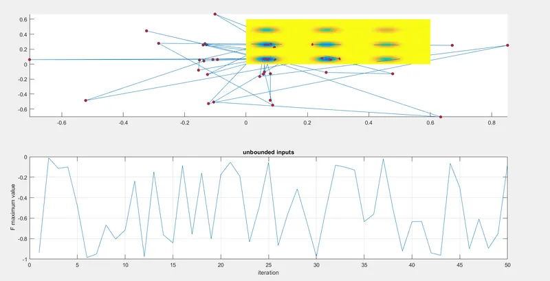
figure(1)
subplot(2,1,1)
hold on
surfc(xx,yy,f)
shading interp
plot3(xopt,yopt,fopt,'marker','o','markersize',5,'markerfacecolor','r')
subplot(2,1,2)
plot(fopt)
title('unbounded inputs')
xlabel('iteration')
ylabel(' F maximum value')
grid on

%% statistical behaviour with upper and lower bound

tic
for i = 1:num_cases
    [input, fopt(i)] = ga(@stalagmite_max,2,[],[],[],[],[0;0],[1;1])
    xopt(i) = input(1)
    yopt(i) = input(2)
end

study_time_2 = toc

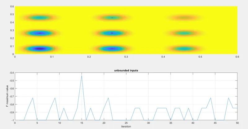
figure(2)
subplot(2,1,1)
hold on
surfc(xx,yy,f)
shading interp
plot3(xopt,yopt,fopt,'marker','o','markersize',5,'markerfacecolor','r')
subplot(2,1,2)
plot(fopt)
title('unbounded inputs')
xlabel('iteration')
ylabel(' F maximum value')
grid on

%% study 3 : increasing ga iterations
tic
options = optimoptions('ga')
options = optimoptions(options,'populationsize',170)

for i = 1:num_cases
    [input, fopt(i)] = ga(@stalagmite_max,2,[],[],[],[],[0;0],[1;1],[],options);
    xopt(i) = input(1)
    yopt(i) = input(2)
    
end

study_time3 = toc

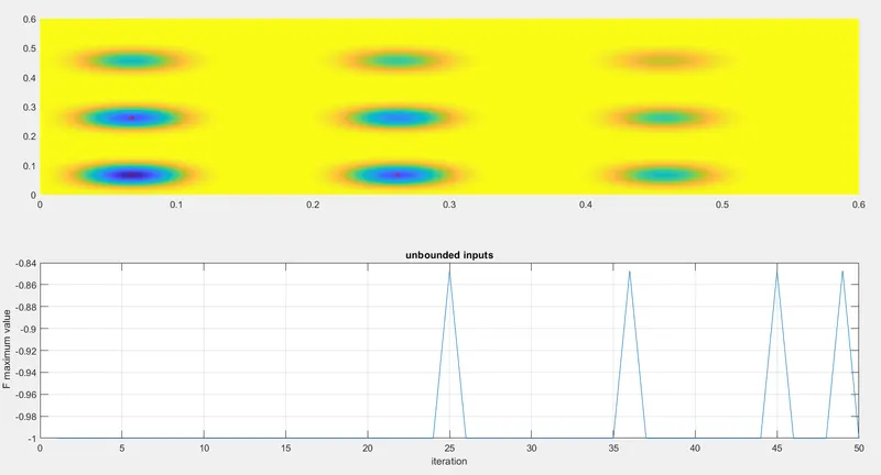
figure(3)
subplot(2,1,1)
hold on
surfc(xx,yy,f)
shading interp
plot3(xopt,yopt,fopt,'marker','o','markersize',5,'markerfacecolor','r')
subplot(2,1,2)
plot(fopt)
title('unbounded inputs')
xlabel('iteration')
ylabel(' F maximum value')
grid on

 

Stalagmite function for max:

function [f] = stalagmite_max(input_s)

x = input_s(1);
y = input_s(2);

f1 = sin(5.1.*pi.*x + 0.5).^6;

f2 = sin(5.1.*pi.*y + 0.5).^6;

f3 = exp(-4*log(2).*(((x - 0.0667).^2)./0.64));

f4 = exp(-4*log(2).*(((y - 0.0667).^2)./0.64));

f = -(f1.*f2.*f3.*f4);  %% to convert min to max function we should multiply with negative sign


end

output: