Week 4.1 - Genetic Algorithm

GENETIC ALGORITHM

AIM: To write a code in MATLAB to optimise the stalagmite function and find the global maxima of the function.

THEORY: A genetic algorithm is a search heuristic that is inspired by Charles Darwin's theory of natural evolution. This algorithm reflects the process of natural selection where the fittest individuals are selected for reproduction in order to produce offspring of the next generation.

The process of natural selection starts with the selection of fittest individuals from a population. They produce offspring which inherit the characteristics of the parents and will be added to the next generation. If parents have better fitness, their offspring will be better than parents and have a better chance at surviving. This process keeps on iterating and at the end, a generation with the fittest individuals will be found.

This notion can be applied for a search problem. We consider a set of solutions for a problem and select the set of best ones out of them.

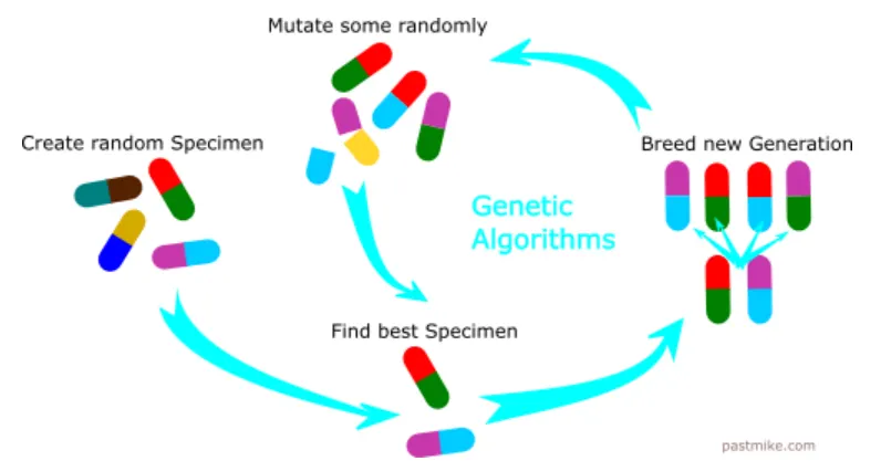
Five phases are considered in a genetic algorithm.

• Initial population-The process begins with a set of individuals which is called a Population. Each individual is a solution to the problem you want to solve.An individual is characterized by a set of parameters (variables) known as Genes. Genes are joined into a string to form a Chromosome (solution).In a genetic algorithm, the set of genes of an individual is represented using a string, in terms of an alphabet. Usually, binary values are used

• Fitness function-The fitness function determines how fit an individual is (the ability of an individual to compete with other individuals). It gives a fitness score to each individual. The probability that an individual will be selected for reproduction is based on its fitness score.

• Selection-The idea of selection phase is to select the fittest individuals and let them pass their genes to the next generation.Two pairs of individuals (parents) are selected based on their fitness scores. Individuals with high fitness have more chance to be selected for reproduction.

• Crossover-Crossover is the most significant phase in a genetic algorithm. For each pair of parents to be mated, a crossover point is chosen at random from within the genes.Offspring are created by exchanging the genes of parents among themselves until the crossover point is reached.The new offspring are added to the population.

• Mutation-In certain new offspring formed, some of their genes can be subjected to a mutation with a low random probability. This implies that some of the bits in the bit string can be flipped.Mutation occurs to maintain diversity within the population premature convergence.

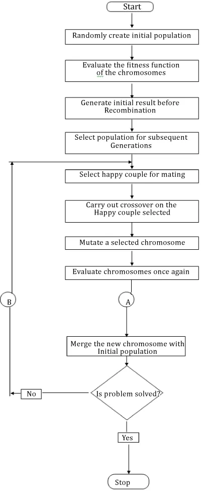
FLOWCHART:

ADVANTAGES OF GA:

• The concept is easy to understand.
• GA search from a population of points, not a single point.
• GA use payoff (objective function) information, not derivatives.
• GA supports multi-objective optimization.
• GA use probabilistic transition rules, not deterministic rules.

APPLICATIONS OF GA:

• Optimization − Genetic Algorithms are most commonly used in optimization problems wherein we have to maximize or minimize a given objective function value under a given set of constraints. The approach to solve Optimization problems has been highlighted throughout the tutorial.

• Economics − GAs are also used to characterize various economic models like the cobweb model, game theory equilibrium resolution, asset pricing, etc.

• Neural Networks − GAs are also used to train neural networks, particularly recurrent neural networks.

• Parallelization − GAs also have very good parallel capabilities, and prove to be very effective means in solving certain problems, and also provide a good area for research.

• Image Processing − GAs are used for various digital image processing (DIP) tasks as well like dense pixel matching.

• Vehicle routing problems − With multiple soft time windows, multiple depots and a heterogeneous fleet.

• DNA Analysis − GAs have been used to determine the structure of DNA using spectrometric data about the sample.

• Multimodal Optimization − GAs are obviously very good approaches for multimodal optimization in which we have to find multiple optimum solutions.

• Traveling salesman problem and its applications − GAs have been used to solve the TSP, which is a well-known combinatorial problem using novel crossover and packing strategies.

The aim of the program is to optimize the stalagmite function

The Stalagmite function is defined as follows:

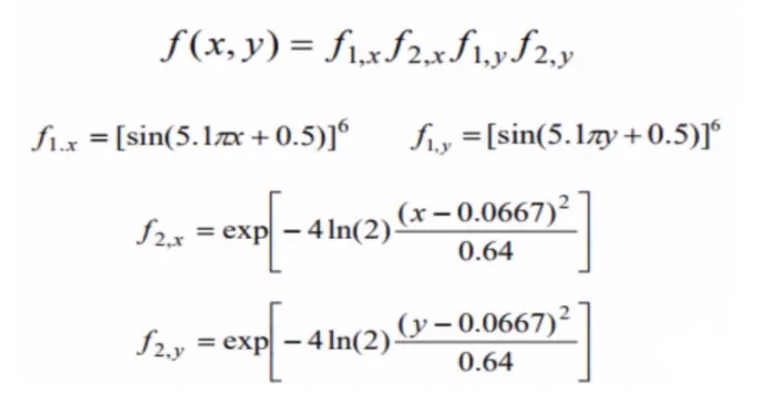
This is the MATLAB code of the Stalagmite function.

function[f]=stalagmite(input_vector) %stalagmite function has the input as input_vector which consists of input variables x and y
x=input_vector(1);
y=input_vector(2);
f1=(sin(5.1*pi*x+0.5))^6;
f2=(sin(5.1*pi*y+0.5))^6;
f3=exp(-4*log(2)*(x-0.0667)^2/0.64);
f4=exp(-4*log(2)*(y-0.0667)^2/0.64);
f=-(f1*f2*f3*f4); %the -ve sign indicates the inverse of the Stalagmite function
end

PROCEDURE:

• The Stalagmite function is defined which is called further in the main body of the GA program
• The x and y values are defined with the 'linspace' command.
• The input vectors are now converted into an array[xx yy] which will make it easier to evaluate a two variable function and also plot 3D mesh/plot.
• The values in these matrices is given as the input to the function created by calling in the main body. By this, we obtain the value of the Stalagmite function at different values of x and y.
• After obtaining the various values of the Stalagmite function, the maxima of the values is obtained by using the 'ga' command which is an inbuilt function in MATLAB.
• The syntax for the GA command is as follows x=ga(fun,nvars,A,b,Aeq,beq,lb,ub,nonlcon,options)
• The number of iterations for which the GA has to run is defined and this is done by using a for loop and the values at each iteration is stored in an array.
• GA in general gives us the minima of the function. As we are interested in finding out the maxima, the Stalagmite function is inversed by using a '-' sign. This provides us the global maxima.
• The study time is thus calculated by using the 'tic' and 'toc' command at the beginning and end of the GA loop respectively.
• The results are plotted using the surfc and the plot commands.
• The GA is made to run for 3 cases, that is, unbounded inputs, bounded inputs and reducing population size.

MATLAB MAIN CODE:

CASE 1: In this case, the behaviour of the algorithm is observed and studied without defining the upper and lower bounds or the search space

clear all
close all
clc
x=linspace(0,0.6,150); % x inputs
y=linspace(0,0.6,150); % y inputs
[xx,yy]=meshgrid(x,y);

%Evaluating the Stalagmite function
for i=1:length(xx);
  for j=1:length(yy); 
      input_vector(1)=xx(i,j);
      input_vector(2)=yy(i,j);
      f(i,j)=stalagmite(input_vector);
  end
end

num_of_iter=50; % GA runs for 50 iterations
tic %study time count start
for i=1:num_of_iter;
    [inputs,f_opt(i)]=ga(@stalagmite,2); %GA function optimizes the Stalagmite function and provides the output
    x_opt(i)=inputs(1);
    y_opt(i)=inputs(2);
    opt_f(i)= -f_opt(i) %GA gives us the minima.Finding the inverse gives us the maxima of the function
end
study_time=toc

%Plotting
subplot(2,1,1)
hold on
surfc(x,y,f) %Generating the Stalagmite function
shading interp %Generates a smooth curve without the mesh grid lines
plot3(x_opt,y_opt,f_opt,'marker','o','markersize',4,'markerfacecolor','r')
title('Unbounded inputs')
subplot(2,1,2)
plot(opt_f)
xlabel('Number of iterations')
ylabel('Max value of function')
      

OUTPUT AND INFERENCE:

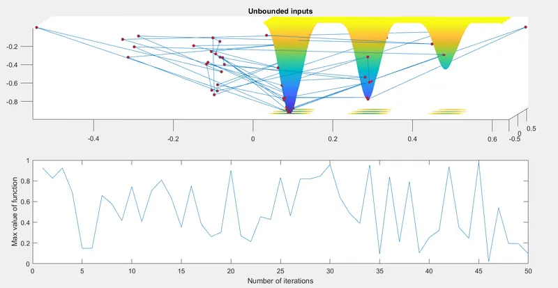
From the above graph we can observe that since we have not defined any bounds to the inputs, the GA algorithm has mapped local maxima points outside the Stalalgmite function. We also cannot obtain a definite value of the global maxima and hence this is not efficient

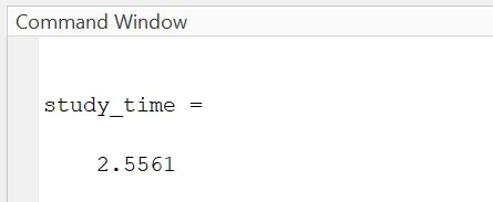
The study time is 2.55s which is very less and the GA algorithm runs only for 50 iterations.

CASE 2: In this case, the lower and upper boundaries are defined inorder within which the global maxima lies. The number of iterations is increased to 100.

clear all
close all
clc
x=linspace(0,0.6,150); % x inputs
y=linspace(0,0.6,150); % y inputs
[xx,yy]=meshgrid(x,y);

%Evaluating the Stalagmite function
for i=1:length(xx);
  for j=1:length(yy); 
      input_vector(1)=xx(i,j);
      input_vector(2)=yy(i,j);
      f(i,j)=stalagmite(input_vector);
  end
end

num_of_iter=100; % GA runs for 50 iterations
tic %study time count start
for i=1:num_of_iter;
    % A,b,Aeq,beq=[] as there are no linear equalities and inequalities
    %lower bounds of the variables x and y are [0,0]
    %upper bounds of the variables x and y are [0.6,0.6]
    [inputs,f_opt(i)]=ga(@stalagmite,2,[],[],[],[],[0;0],[0.6;0.6]); %GA function optimizes the Stalagmite function and provides the output
    x_opt(i)=inputs(1);
    y_opt(i)=inputs(2);
    opt_f(i)= -f_opt(i) %GA gives us the minima.Finding the inverse gives us the maxima of the function
end
study_time=toc

%Plotting
subplot(2,1,1)
hold on
surfc(x,y,f) %Generating the Stalagmite function
shading interp %Generates a smooth curve without the mesh grid lines
plot3(x_opt,y_opt,f_opt,'marker','o','markersize',4,'markerfacecolor','r')
title('Bounded inputs')
subplot(2,1,2)
plot(opt_f)
xlabel('Number of iterations')
ylabel('Max value of function')
      

OUTPUT AND INFERENCE:

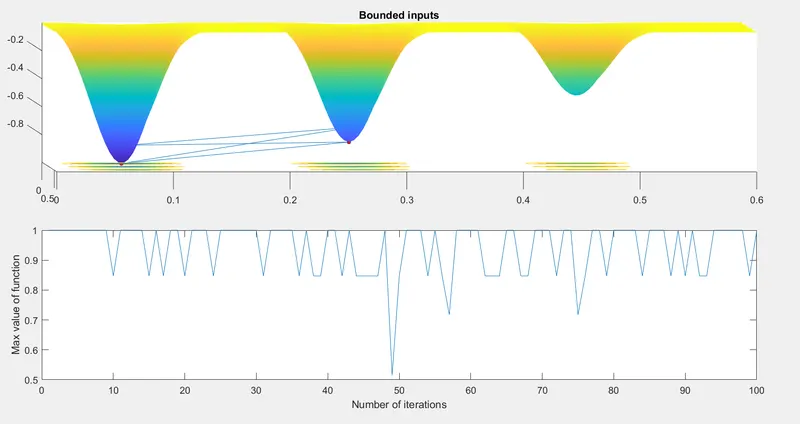
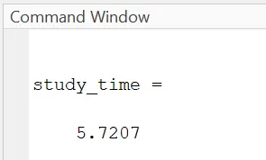
The above graph is much more optimized compared to the first case as the boundaries within which the global maxima exists is defined. This graph gives a much clearer range about where the global maxima exists.

CASE 3: In this case, the population size is increased so as to converge to the global maxima

clear all
close all
clc
x=linspace(0,0.6,150); % x inputs
y=linspace(0,0.6,150); % y inputs
[xx,yy]=meshgrid(x,y);

%Evaluating the Stalagmite function
for i=1:length(xx);
  for j=1:length(yy); 
      input_vector(1)=xx(i,j);
      input_vector(2)=yy(i,j);
      f(i,j)=stalagmite(input_vector);
  end
end

num_of_iter=150; % GA runs for 50 iterations

options=optimoptions('ga');
options=optimoptions(options,'populationsize',450);

tic %study time count start
for i=1:num_of_iter;
    % A,b,Aeq,beq=[] as there are no linear equalities and inequalities
    %lower bounds of the variables x and y are [0,0]
    %upper bounds of the variables x and y are [0.6,0.6]
    [inputs,f_opt(i)]=ga(@stalagmite,2,[],[],[],[],[0;0],[0.6;0.6],[],options); %GA function optimizes the Stalagmite function and provides the output
    x_opt(i)=inputs(1);
    y_opt(i)=inputs(2);
    opt_f(i)= -f_opt(i) %GA gives us the minima.Finding the inverse gives us the maxima of the function
end
study_time=toc

%Plotting
subplot(2,1,1)
hold on
surfc(x,y,f) %Generating the Stalagmite function
shading interp %Generates a smooth curve without the mesh grid lines
plot3(x_opt,y_opt,f_opt,'marker','o','markersize',4,'markerfacecolor','r')
title('Bounded inputs')
subplot(2,1,2)
plot(opt_f)
xlabel('Number of iterations')
ylabel('Max value of function')
      

OUTPUT AND INFERENCE:

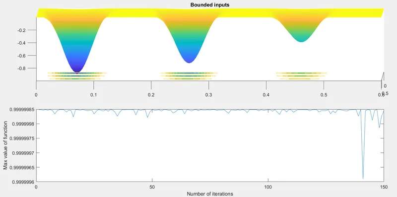
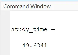
In this case we can observe that the global maxima has converged at one point and hence we obtain a specific value. Since the number of iterations and the population have been significantly increased, subsequently the study time also increases.

ERRORS:

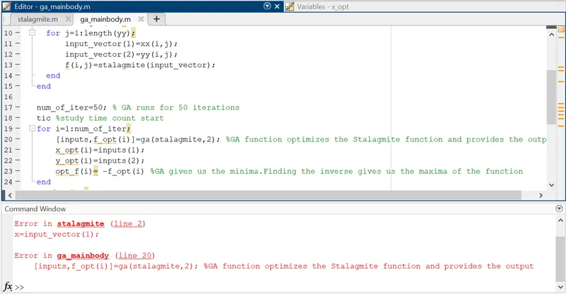
The error here was the incorrect usage of the GA syntax. I forgot to add the '@'. This was rectified by using [inputs,f_opt(i)]=ga(@stalagmite,2);

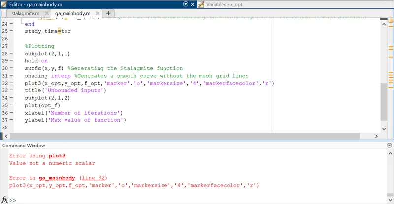
This was the second error. The error here was quoting the markersize 4 which is an improper syntax. This was rectified using plot3(x_opt,y_opt,f_opt,'marker','o','markersize',4,'markerfacecolor','r')

CONCLUSION: Thus we can conclude that the GA algorithm gives us accurate results when provided with bounded inputs and on increasing the population size and the number of iterations for which the GA runs.