Project 1 - Parsing NASA thermodynamic data

PARSING NASA THERMODYNAMIC DATA

AIM: To write a MATLAB code inorder to parse the NASA thermodynamic data and thus calculate the thermodynamic properties of various gases.

OBJECTIVE:

• Write a function that extracts the 14 co-efficients and calculates the enthalpy, entropy and specific heats for all the species in the data file.
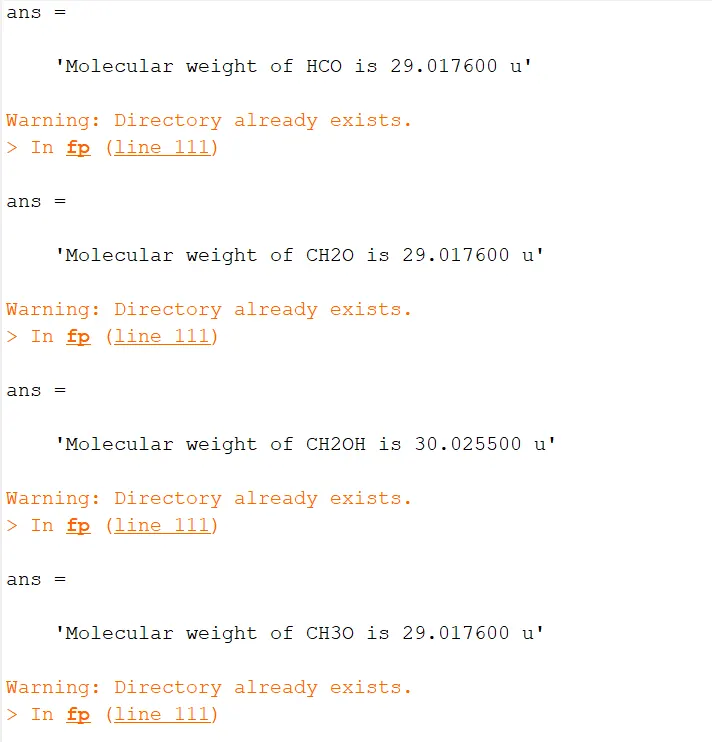
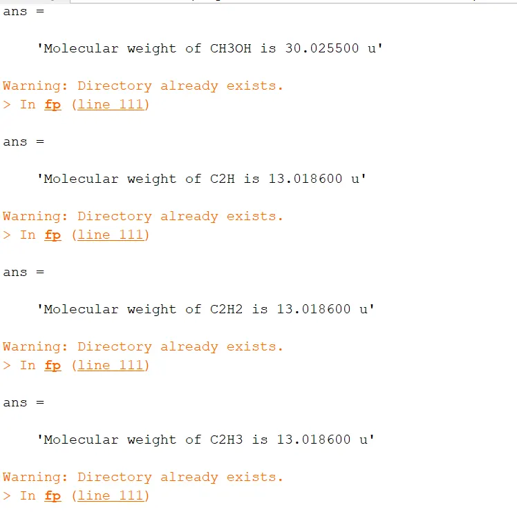
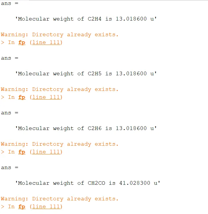
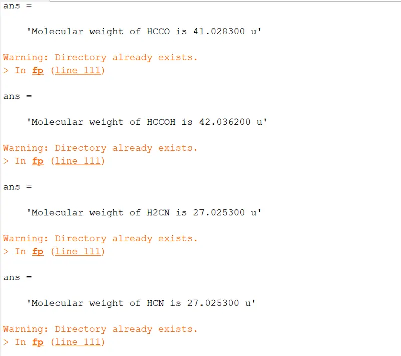
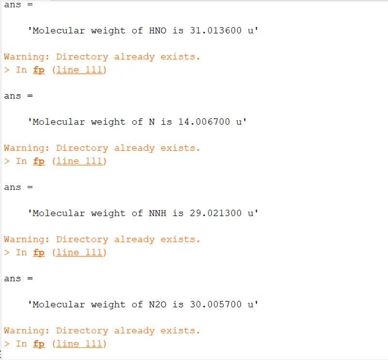
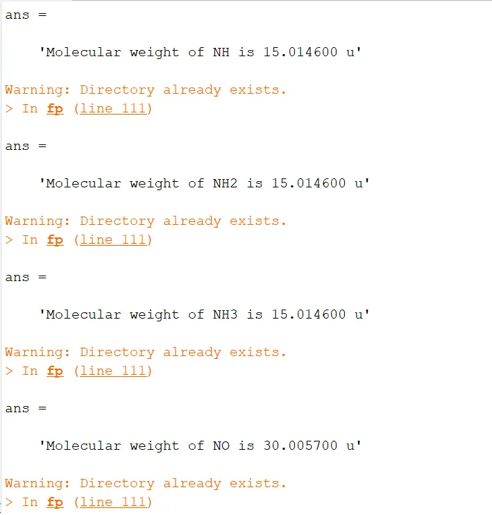
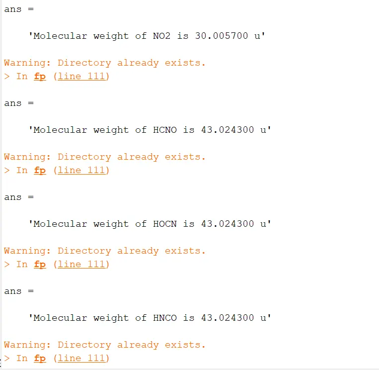
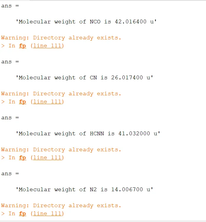
• To calculate the molecular weight of each species and display it in the command window.
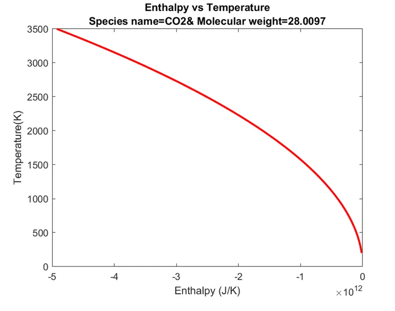
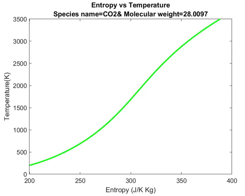
• Plot the Cp, Enthalpy and Entropy for the local temperature range (low temperature : high temperature) specific for each species.

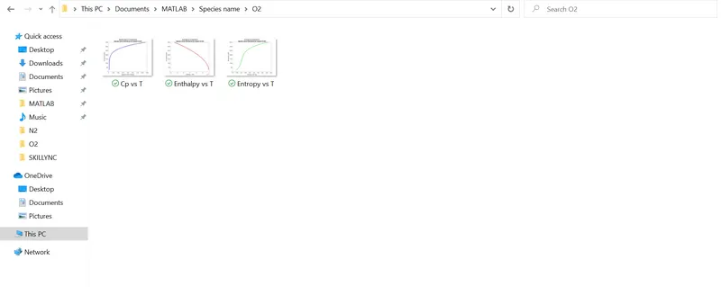
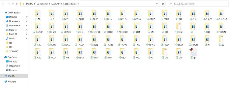
• Save the plots as images with appropriate names and dump them in separate folders for each species with suitable name. All these should be generated automatically.

• The main program that you will submit will just take the "THERMO.dat" file as an input and generate Cp, H and S plots.

THEORY:

FILE PARSING: Parsing, syntax analysis, or syntactic analysis is the process of analyzing a string of symbols, either in natural language, computer languages or data structures, conforming to the rules of a formal grammar.Parsing a file means reading in a data stream of some sort and building an in memory model of the semantic content of that data. This aims at facilitating perfoming some kind of transformation on the data.It can be used to describe split or separation.

SPECIFIC HEAT: Specific heat, the quantity of heat required to raise the temperature of one gram of a substance by one Celcius degree. The units of specific heat are usually calories or joules per gram per Celsius degree.

ENTROPY: A thermodynamic quantity representing the unavailability of a system's thermal energy for conversion into mechanical work, often interpreted as the degree of disorder or randomness in the system.

ENTHALPY: Enthalpy is a property of a thermodynamic system, and is defined as the sum of the system's internal energy and the product of its pressure and volume. It is a state function used in many measurements in chemical, biological, and physical systems at a constant pressure.The unit of measurement for enthalpy in the SI unit system is Joule.

GAS CONSTANT: The gas constant is a physical constant denoted by R and is expressed in terms of units of energy per temperature increment per mole. It is also known as Ideal gas constant or molar gas constant or universal gas constant. The gas constant value is equivalent to Boltzmann constant but expressed as the pressure-volume product instead of energy per increment of temperature per particle.The ideal gas constant is the combination of Boyle’s law, Avogadro’s number, Charles’s law and Gay-Lussac’s law.

Gas constant R = 8.3144598(48) J⋅mol⁻¹⋅K^−1\

NASA SAMPLE THERMODYNAMIC DATA:

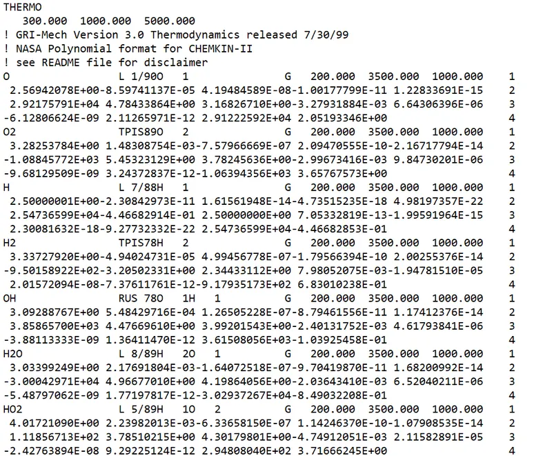
Where,

Cp= Specific heat((J/K Kg)

R=Universal gas constant (8.314 J/K.mol)

H=Enthalpy(J)

S=Entropy(J/K)

T=Temperature(K)

MATLAB CODE:

clear all
close all
clc

f1=fopen('THERMO.dat','r') ;%file reading
for j=1:5
    fgetl(f1);%reading the lines
end
%Extracting species data
for i=1:53
    
    %extracting the name of gas species
    A=fgetl(f1); %reading the 5th line
    z=strsplit(A,' '); %reading the species line
    species_name= z{1};
 
    %extraction of local Terature of gas species
    
    a=strfind(A,'.'); %Finding string from the line
    t1=A((a(1)-3):a(1)+3); %assigning 't' variable for local Terature
    low_local_T=str2double(t1); %converting string to variable
    t2=A((a(3)-4):a(3)+3);
    mid_local_T=str2double(t2); 
    t3=A((a(2)-4):a(2)+3); 
    high_local_T=str2double(t3);
    %t1= low Terature
    %t2= mid Terature
    %t3= high Terature
    
    %Extracting co-efficient of gas species
    B=fgetl(f1);
    b=strfind(B,'E');
    a1=B(1:b(1)+3); %Assigning 'A' variable for Terature coefficients
    a1=str2double(a1);
    a2=B(b(1)+4:b(2)+3);
    a2=str2double(a2);
    a3=B(b(2)+4:b(3)+3);
    a3=str2double(a3);
    a4=B(b(3)+4:b(4)+3);
    a4=str2double(a4);
    a5=B(b(4)+4:b(5)+3);
    a5=str2double(a5);
    C=fgetl(f1);
    c=strfind(C,'E');
    a6=C(1:c(1)+3); 
    a6=str2double(a6);
    a7=C(c(1)+4:c(2)+3);
    a7=str2double(a7);
    a8=C(c(2)+4:c(3)+3);
    a8=str2double(a8);
    a9=C(c(3)+4:c(4)+3);
    a9=str2double(a9);
    a10=C(c(4)+4:c(5)+3);
    a10=str2double(a10);
    D=fgetl(f1);
    d=strfind(D,'E');
    a11=D(1:d(1)+3); 
    a11=str2double(a11);
    a12=D(d(1)+4:c(2)+3);
    a12=str2double(a12);
    a13=D(d(2)+4:c(3)+3);
    a13=str2double(a13);
    a14=D(d(3)+4:c(4)+3);
    a14=str2double(a14);
    
    %First 7 are high Terature co-efficients from a1 to 7
    %Second 7 are low Terature co-efficients from a8 to 14
    
    %To create the range of low and high values of local Terature
    
    T=linspace(low_local_T,high_local_T,1000);
    R=8.314; %Universal gas constant
    
    %Calculation for Specific heat, Enthalpy and Entropy
   
    
     
    if T>mid_local_T
    Cp = R*(a1 + a2*(T) + a3*((T).^2) + a4*((T).^3) + a5*((T).^4));
    H = (R*T).*(a1 + (a2*T/2) + (a3*(T.^2)/3) + (a4*(T.^3)/4) + (a5*(T.^4)/5) + (a6*(T)));
    S = R*(a1*log(T) + a2*(T) + ((a3*(T).^2)/2) + ((a4*(T).^3)/3) + ((a5*(T).^4)/4) + a7);
    else
    Cp = R*(a8 + a9*(T) + a10*((T).^2) + a11*((T).^3) + a12*((T).^4));
    H = (R*T).*((a8 +(a9*T/2))+ ((a10*(T).^2)/3) + ((a11*(T).^3)/4)+((a12*(T).^4)/5) + (a13*(T)));
    S = R*(a8*log(T) + a9*(T) + ((a10*(T).^2)/2) + ((a11*(T).^3)/3) + ((a12*(T).^4)/4) + a14);
    end  
    
    
    %Molecular weight calculation
    elements=['H','C','O','N','A','S'] %Declaring species element
    atomic_weight=[1.0079 12.0107 15.999 14.0067 39.948 32.065]; %Declaing the atomic values
    mol_mass=0; %Declaring molecular mass to be initially 0
    
    for l=1:length(species_name)
        for m=1:length(atomic_weight)
            if strcmp(species_name(l),elements(m))
                mol_mass=mol_mass+atomic_weight(m);
                position=m;
            end
        end
        n=str2double(species_name(1));
        if n>1
            mol_mass=mol_mass+atomic_weight(position)*(n-1);
        end
    end
    
    %Printing molecular weight of the gas species
    sprintf('Molecular weight of %s is %f u',species_name,mol_mass)
    
    %Creating a folder to save the files
    mkdir(['C:\Users\phalg\OneDrive\Documents\MATLAB\Species name\',species_name]) %Creating a new folder with the species name
    
    
    %Plotting specific heat vs Terature
     figure(1)
     plot(Cp,T,'color','b','linewidth',2)
     ylabel('Temeperature(K)')
     xlabel('Specific heat (J/K Kg)')
     title({'Specific heat vs Terature',['Species name=',species_name,'& Molecular weight=',num2str(mol_mass)]});
     
    
     %Plotting enthalpy vs Terature
     figure(2)
     plot(H,T,'color','r','linewidth',2)
     ylabel('Temeperature(K)')
     xlabel('Enthalpy (J/K)')
     title({'Enthalpy vs Terature',['Species name=',species_name,'& Molecular weight=',num2str(mol_mass)]});
     
     
     %Plotting entropy vs Terature
     figure(3)
     plot(S,T,'color','g','linewidth',2)
     ylabel('Temeperature(K)')
     xlabel('Entropy (J/K Kg)')
     title({'Entropy vs Terature',['Species name=',species_name,'& Molecular weight=',num2str(mol_mass)]})
     cd(['C:\Users\phalg\OneDrive\Documents\MATLAB\Species name\',species_name])
     saveas(figure(1),'Cp vs T.png')
     saveas(figure(2),'Enthalpy vs T.png')
     saveas(figure(3),'Entropy vs T.png')
     
        
end
fclose(f1);

PROGRAM EXPLANATION:

• The code is always began with 'clear all', 'close all' and 'clc' inorder to clear the workspace and the command window for preventing the over writing of programs.
• The 'THERMO.dat' file is opened for reading the external NASA data using the fopen command and this is assigned the value of f1.
• The fgetl(f1) command is used to read the data line by line and acts like a line cursor.
• The next five lines have been to skipped inorder to obtain the pattern of the gas species. This is done by initializing the for loop to obtain the data pertaining to all the gas species.
• The name of the gas species is found out using the 'findstr' command and inorder to find the species, we are going to locate the string ' ' which will be the distinguishing factor.
• Declaring 'species_name= z{1}', gives us the location of the species name and further the name of the gas species is stored in the variable 'species_name'.
• The local temperatures of the respective gases is similarly found using findstr command and this is located using the string '.' by which we obtain the values of low temperature,mid temperature and high temperature which are assigned the variables t1, t2 and t3 respectively.
• The obtained values are in the string format. Hence they are converted to numbers using the 'str2double' command.
• The next step is to extract the co-efficient values of the gas species similarly how it was done for obtaining the local temperature values. They are extracted using the commands 'findstr' and 'str2double' and stored in the variables from a1 to a14.
• For extracting, we are going to locate the string 'E' which is present in every co-efficient value and this is further carried on for all the co-efficients in the same line and the successor lines.
• The values from a1 to a7 represent high temperatures and from a8 to 14 represent the low temperatures.
• The temperature value range is initialized using the 'linspace' command.
• The values of specific heat, enthalpy and entropy are calculated in accordance with the formula. Further, the if else command is used to determine if the temperature value is lesser or greater than the mid temperature.
• Inorder to calculate the molecular weight, the element cell array is defined consisting of the species elements. Their respective atomic weights are declared in another array. The molecular weight is initialized to 0.
• Now, the for loop is used to detect the presence of more than one species in the variable species_name and it's respective gas species values are calculated.
• After the nested for loop, the species name is converted to a number using the 'str2double' command. The molecular weight is now calculated again by having the value of the atomic weight for the current species and displayed on the command window.
• The plots are created for the obtained values of specific heat, enthalpy and entropy and saved in the folder species_name automatically.
• We make use of the command 'mkdir' to make a new folder with the species_name which is in the main folder. Now the 'cd' command is used to change the current directory from the main folder to the species_name.
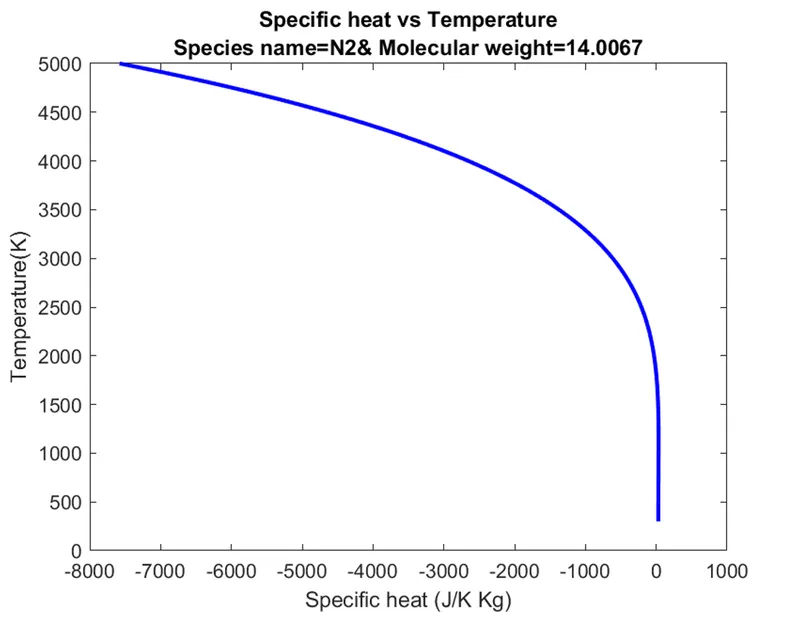
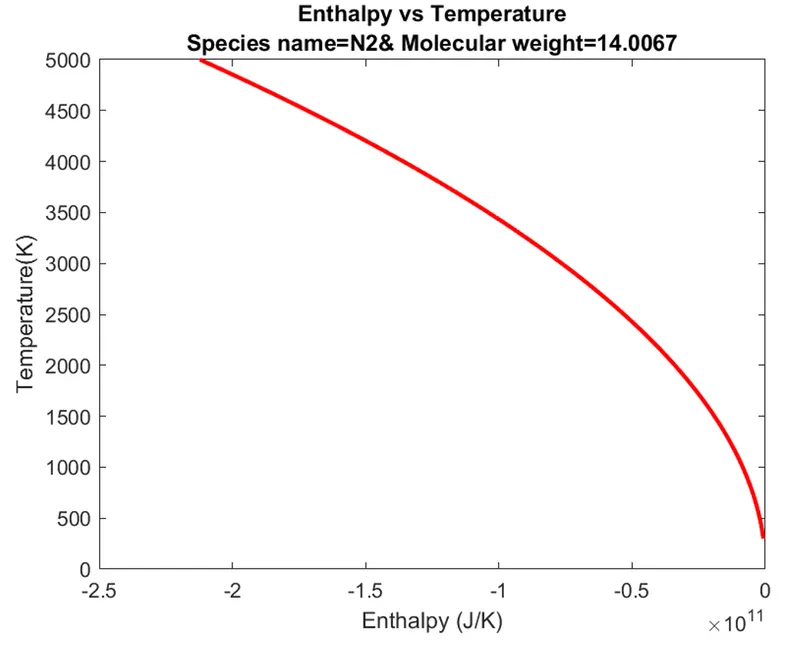
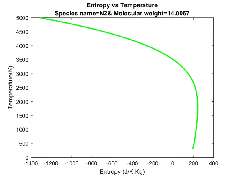
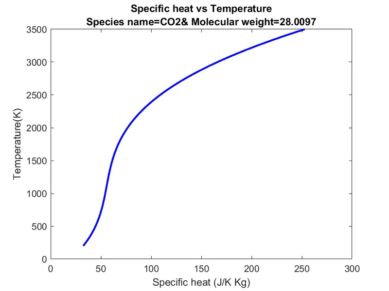
• The plots for specific heat vs temperature, enthalpy vs temperature and entropy vs temperature is plotted and the axis are labelled accordingly along with the molecular weight value.
• Inorder to save the plots, the 'saveas' command is used to save in the current folder.

OUTPUTS:

O2 PLOT:

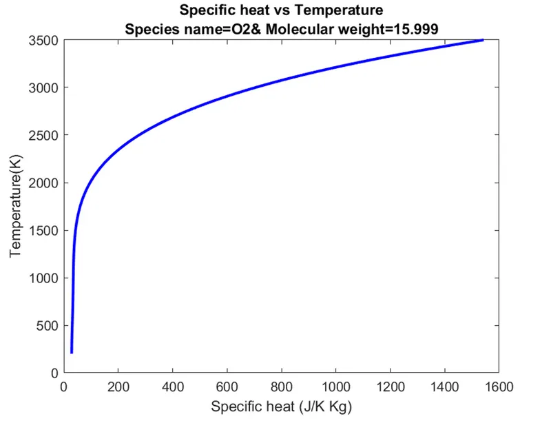
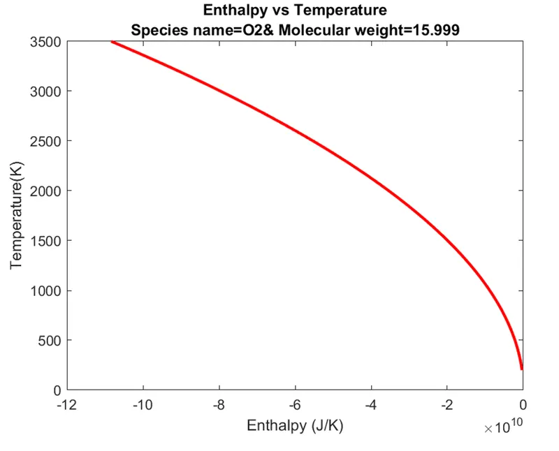
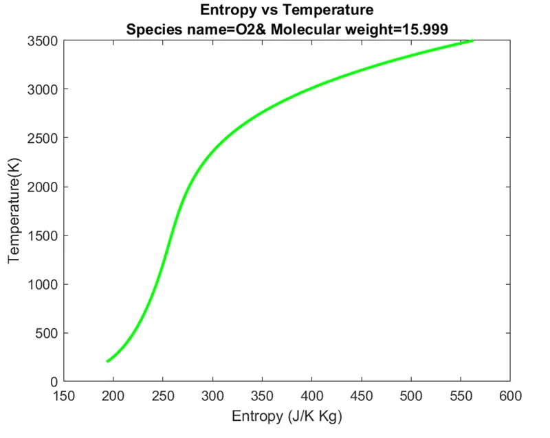
N2 PLOT:

CO2 PLOT:

FOLDER CONTAINING THE PLOTS:

FOLDER CONTAINING ALL THE SPECIES:

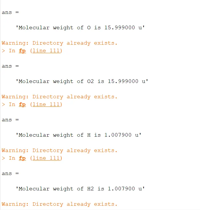
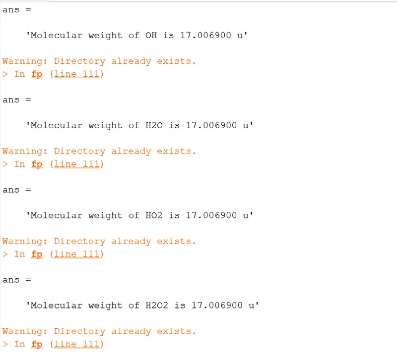
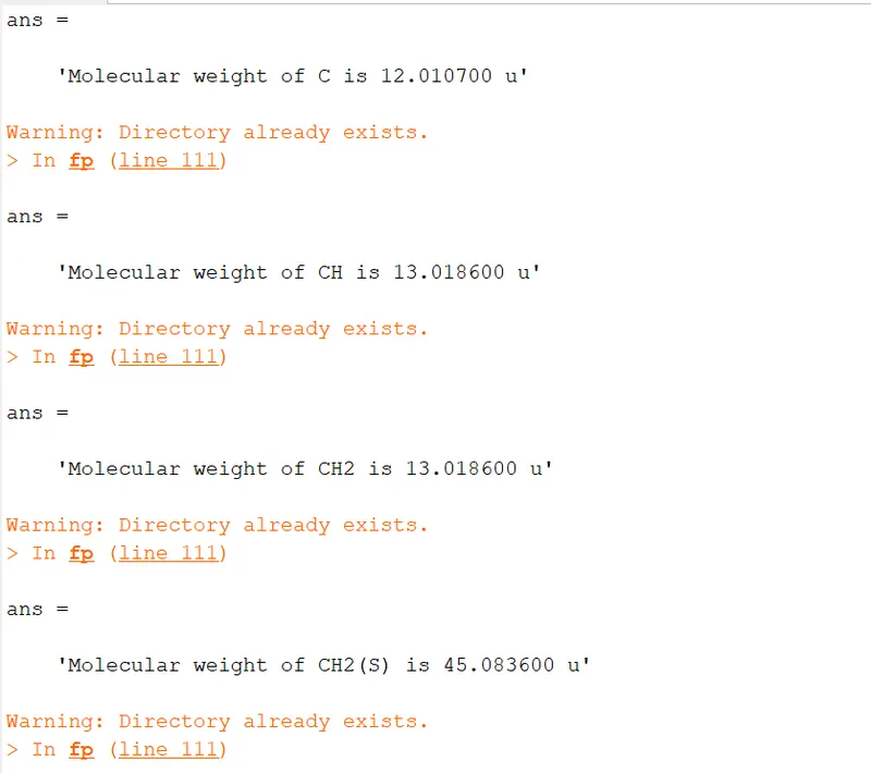
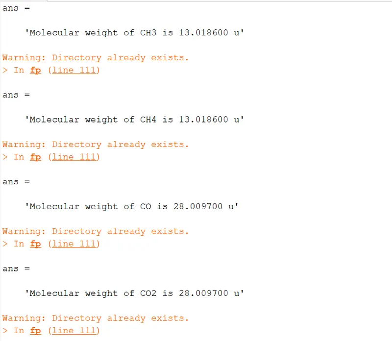
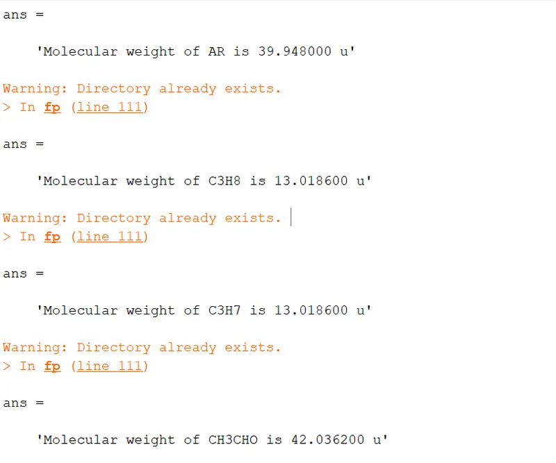
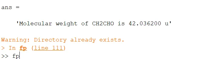
MOLECULAR WEIGHT OF ALL THE SPECIES DISPLAYED IN THE COMMAND WINDOW:

ERRORS FACED:

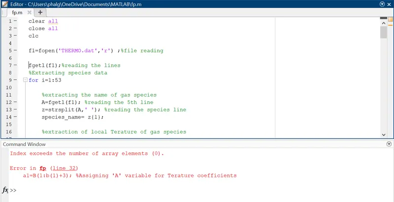
1. The first error faced was by not adding THERMO.dat into the same while where the MATLAB code exists. This was rectified by adding it to the same path.
2. The second error was the program was'nt reading the lines from the 5th line. This was solved by initializing a for loop which skipped the 5 lines and read the species line.

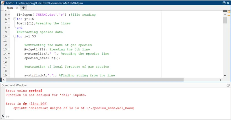
3. The third error was the improper usage of brackets to define a cell. This was rectified by replacing the paranthesis with the curly brackets.

SPECIES NAME FOLDER LINK: https://1drv.ms/u/s!Agr4OI-5Q-gCgkeUzGK8ridJX9BN?e=6yqZeJ

CONCLUSION: The given NASA thermodynamic data has been successfully parsed and the graphs of specific heat vs temperature, enthalpy vs temperature and entropy vs temperature of all the gas species have been plotted.