Week 3 - Solving second order ODEs

SOLVING SECOND ORDER ODE

AIM: To write a program that solves the following ODE representing the equation of motion of a simple pendulum with damping and to create a plot between angular displacement and velocity by using ode45 command. The animation of the above has to be created.

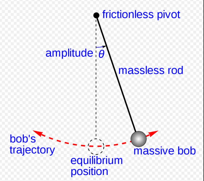
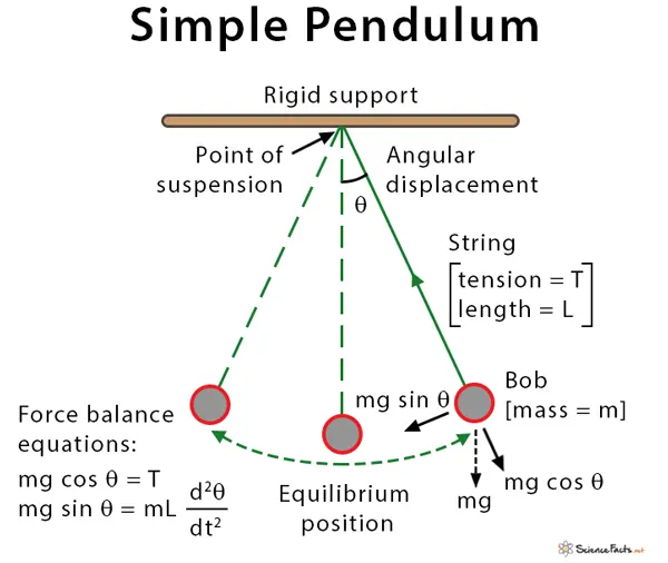
• g = gravity in m/s2,
• L = length of the pendulum in m,
• m = mass of the ball in kg,
• b=damping coefficient

THEORY:

ORDINARY DIFFERENTIAL EQUATION(ODE): In mathematics, an ordinary differential equation (ODE) is a differential equation containing one or more functions of one independent variable and the derivatives of those functions. The term ordinary is used in contrast with the term partial differential equation which may be with respect to more than one independent variable.

where is a function of , is the first derivative with respect to , and is the th derivative with respect to

SIMPLE HARMONIC MOTION OF A PENDULUM: In mechanics and physics, simple harmonic motion is a special type of periodic motion where the restoring force on the moving object is directly proportional to the object's displacement magnitude and acts towards the object's equilibrium position. It results in an oscillation which, if uninhibited by friction or any other dissipation of energy, continues indefinitely.Simple harmonic motion can serve as a mathametical model for a variety of motions.

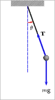
A simple pendulum is one which can be considered to be a point mass suspended from a string or rod of negligible mass. It is a resonant system with a single resonant frequency.

OBJECTIVE:

The above shown 2nd order differential equation gives us the position of the pendulum of the bob at any given instant of time. This can be solved by MATLAB. But MATLAB does not have any function to solve a second order D.E directly. Hence, a 2nd order D.E can be manipulated such that we obtain two first order D.E's and this can be solved in MATLAB by using the function 'ode45'.

Conversion of a 2nd order D.E to 1st order D.E

• Consider θ as the angular displacement. Let θ=θ1
• The differential of angular displacement is angular velocity.

dθ1/dt=θ2. This is the first D.E

• The second one is obtained by differentiating θ2 with respect to time

dθ2/dt= -(b/m)*θ2 - (g/l)sinθ1.This is the second D.E

• Both these 1st order differential equations can be represented in the form of solution matrix.

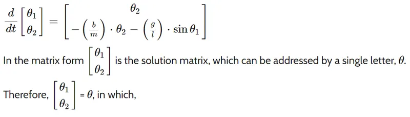
θ1=angular position of the pendulum at various instances of time.

θ2=corresponding angular velocity at the same instances of time.

• The function 'ode45' solves the input and returns 2 sets of values. One is the time which has been given as the input and the second is the matrix θ which has been defined. The second output θ has two columns.The first colums provides us the angular displacement and the second column, the corresponding angular velocity.

MATLAB CODE:

MAIN PROGRAM:

clear all
close all
clc 

%Input parameters
b=0.05; %Damping factor
g=9.81; %Acceleration due to gravity
l=1;    %Length of the pendulum
m=0.1;  %Mass of the pendulum

%initial conditions
theta_0=[0;5]; 

%time points
t_span=linspace(0,30,500);

%solve ode
[t,results]=ode45(@(t,theta) ode_func(t,theta,b,g,l,m),t_span,theta_0);

%Plotting of angular velocity and displacement

figure(1)
plot(t,results(:,1))
hold on
plot(t,results(:,2))
grid on
title('Motion of the pendulum')
ylabel('Angular velocity(rad/sec)/Displacenent(rad)')
xlabel('time in seconds')
legend('Displacement','Angular velocity')

angle=results(:,1);

%Count command for iteration
ct=1;
for i=1:length(angle)
    omega=angle(i);
    figure(2)
    title('Motion of the pendulum')
    
    %To fix coordinates of one end of the simple pendulum
    x0=0;
    y0=0;
    
    %coordinates of the bob
    x1=1*cos((3*pi/2)+omega);
    y1=1*sin((3*pi/2)+omega);
    
    %Plotting the bob motion
    plot([x0 x1],[y0 y1],'linewidth',3,'color','g')
    hold on;
    plot(x1,y1,'o','markers',15,'MarkerFaceColor','k')
    hold on;
    plot([-3 3],[0,0],'linewidth',2,'color','b')
    hold off
    axis([-3 3 -2 2])
    grid on
    pause(0.1)
    M(ct)=getframe(gcf);
    ct=ct+1;
end

%To create an animation of the simple pendulum
movie(M)
videofile=VideoWriter('simple_pendulum.avi','Uncompressed AVI');
open(videofile)
writeVideo(videofile,M)
close(videofile)    

ODE FUNCTION PROGRAM:

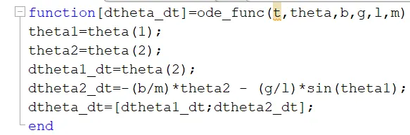
function[dtheta_dt]=ode_func(t,theta,b,g,l,m)
theta1=theta(1);
theta2=theta(2);
dtheta1_dt=theta(2);
dtheta2_dt=-(b/m)*theta2 - (g/l)*sin(theta1);
dtheta_dt=[dtheta1_dt;dtheta2_dt]
end

PROGRAM EXPLANATION:

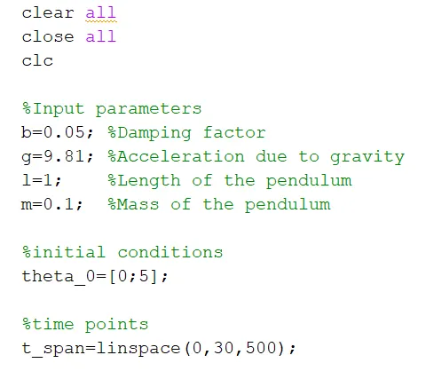
• The 'clear all','close all','clc' commands are used to clear the workspace,command window, previously existing graphs and prevent the over writing of programs.
• The inputs for the pendulum are declared which are

b(Damping factor)=0.05N-m/s

g(Acceleration due to gravity)=9.8m/s

l(Length of the pendulum)=1m

m(Mass of the pendulum)=0.1kg

• t_span is used in the ode45 solver which specifies the time span of the iterations required to solve the O.D.E.
• Initial values for position and velocity are defined

• The 'ode45' function is called. ode45 is function in MATLAB that solves ordinary or partial differential equations using numerical method. Here since the order of the equation is 2, the function should take atleast two inputs to solve the D.E and to obtain the approximate result.
• The syntax of the 'ode45' solver is:

[t,results]=ode4([@(t,y)ode(t,y,args),t_span,y0)

• Following the above syntax, we provide our input parameters and this returns us a matrix of θ2 and dθ2/dt.

• The function 'ode45' accepts the input value and gives two outputs in the form of a matrix after integration. The output is the matrix of angular displacement θ1 and angular velocity θ2.
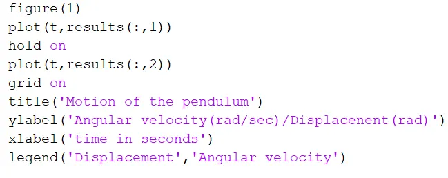
• From the obtained values, a plot of displacement and velocity vs time is plotted. This curve can be manipulated by changing the values of damping factor.The angular velocity and displacement comes to rest at the end of the function.
• The'label' command is used to name the X and Y axis.
• The 'legend' command is used to indicate angular displacement and velocity in the plot.

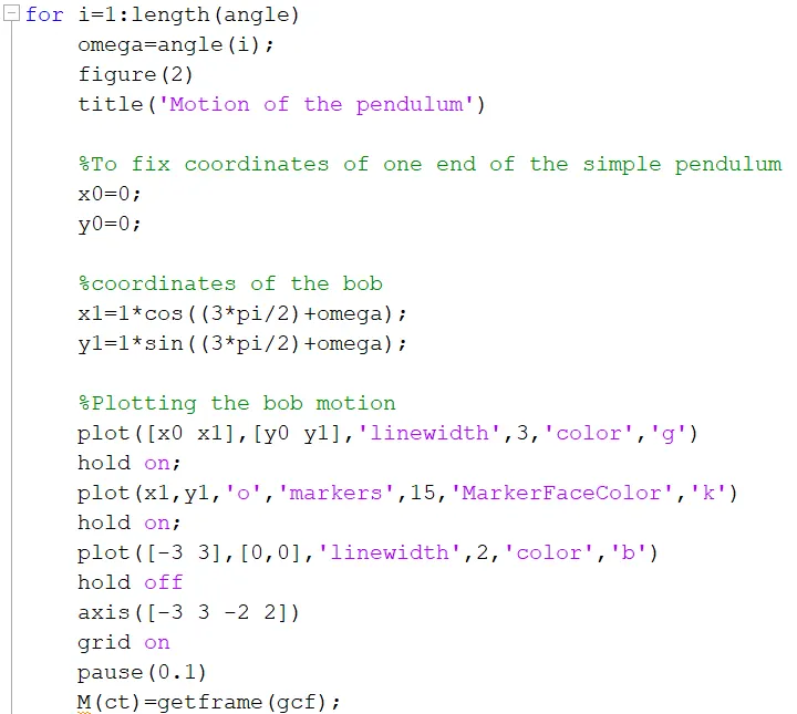
• Now we initialize a counter. A 'for' loop is initialized to plot the position of the bob at every interval. Whenever the for loop increments the counter, the next position of the pendulum is obtained.
• X0 and Y0 are the fixed points at one end and X1 and Y1 is the position of the bob at the different time intervals.

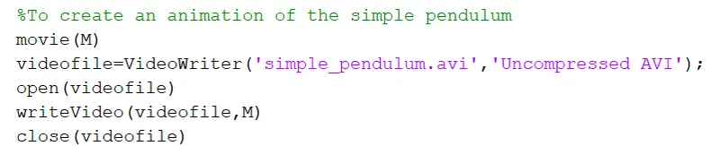
• On exiting the for loop, a movie of the acquired plots is created using the below syntax

• The next step is to create the function 'ode_func(t,theta,b,g,l,m)'
• In a new script, a function is created with return value being 'dtheta_dt
• The input values to this function are t,theta,b,g,l and m respectively.
• In the body of this function, we calculate θ2 and dθ2/dt which are assigned to the elements of the matrix dtheta_dt.
• This matrix is returned to the main program where this function is called.

OUTPUT:

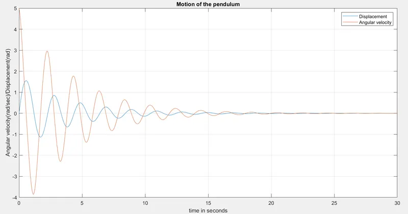
• Here, the displacement starts from 0 and the angular velocity starts from 5rad/sec
• As the time advances that is at the end of t_span, the displacement and the angular velocity becomes zero as the motion of the pendulum comes to rest.

ERROR:

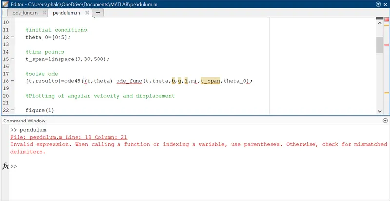
In line 18, the function 'ode45' is not defined in accordance to the syntax as t and theta are not called.

Therefore, the correct syntax would be ' [t,results]=ode45(@(t,theta) ode_func(t,theta,b,g,l,m),t_span,theta_0);'

CONCLUSION:

The simple pendulum is animated using the command 'ode45' where the second order differential equation is reduced to a simpler differential equation which is solvable.

Pendulum animation link-https://1drv.ms/v/s!Agr4OI-5Q-gCgRvGUTA4K6N6KjId?e=txYcf8