Week 4.1 - Genetic Algorithm

Aim:

To write the code to calculate the global maxima of the stalagmite function and to explain the syntax for genetic algoritham(ga) in MATLAB.

Objectives:

• To write a code in MATLAB to optimize the stalagmite function and find global maxima of the function.
• To explain the concept of genetic algoritham and the syntax for ga in MATLAB.
• To plot the graph of all three studies and also for global maxima.

Genetic Algorithm

“Select The Best, Discard The Rest”

The genetic algorithm repeatedly modifies a population of individual solutions. At each step, the genetic algorithm selects individuals at random from the current population to be parents and uses them to produce the children for the next generation.

The genetic algorithm uses three main types of rules at each step to create the next generation from the current population:

• Selection rules select the individuals, called parents, that contribute to the population at the next generation.
• Crossover rules combine two parents to form children for the next generation.
• Mutation rules apply random changes to individual parents to form children.

Syntax for GA

x = ga(fun,nvars)

x = ga(fun,nvars,A,b)

x = ga(fun,nvars,A,b,Aeq,beq)

x = ga(fun,nvars,A,b,Aeq,beq,lb,ub)

x = ga(fun,nvars,A,b,Aeq,beq,lb,ub,nonlcon)

x = ga(fun,nvars,A,b,Aeq,beq,lb,ub,nonlcon,options)

x = ga(fun,nvars,A,b,Aeq,beq,lb,ub,nonlcon,intcon)

x = ga(fun,nvars,A,b,Aeq,beq,lb,ub,nonlcon,intcon,options)

x = ga(problem)

[x,fval] = ga(___)

[x,fval,exitflag,output] = ga(___)

[x,fval,exitflag,output,population,scores] = ga(___)

x = ga(fun,nvars) finds a local unconstrained minimum, x, to the objective function, fun. nvars is the dimension (number of design variables) of fun.

x = ga(fun,nvars,A,b) finds a local minimum x to fun, subject to the linear inequalities A*x ≤ b. ga evaluates the matrix product A*x as if x is transposed (A*x').

x = ga(fun,nvars,A,b,Aeq,beq) finds a local minimum x to fun, subject to the linear equalities Aeq*x = beq and A*x ≤ b. (Set A=[] and b=[] if no linear inequalities exist.) ga evaluates the matrix product Aeq*x as if x is transposed (Aeq*x').

x = ga(fun,nvars,A,b,Aeq,beq,lb,ub) defines a set of lower and upper bounds on the design variables, x, so that a solution is found in the range lb ≤ x ≤ ub. (Set Aeq=[] and beq=[] if no linear equalities exist.)

x = ga(fun,nvars,A,b,Aeq,beq,lb,ub,nonlcon) subjects the minimization to the constraints defined in nonlcon. The function nonlcon accepts x and returns vectors C and Ceq, representing the nonlinear inequalities and equalities respectively. ga minimizes the fun such that C(x) ≤ 0 and Ceq(x) = 0. (Set lb=[] and ub=[] if no bounds exist.)

x = ga(fun,nvars,A,b,Aeq,beq,lb,ub,nonlcon,options) minimizes with the default optimization parameters replaced by values in options. (Set nonlcon=[] if no nonlinear constraints exist.) Create options using optimoptions.

x = ga(fun,nvars,A,b,Aeq,beq,lb,ub,nonlcon,intcon) or x = ga(fun,nvars,A,b,Aeq,beq,lb,ub,nonlcon,intcon,options) requires that the variables listed in intcon take integer values.

x = ga(problem) finds the minimum for problem, a structure described in problem.

[x,fval] = ga(___), for any previous input arguments, also returns fval, the value of the fitness function at x.

[x,fval,exitflag,output] = ga(___) also returns exitflag, an integer identifying the reason the algorithm terminated, and output, a structure that contains output from each generation and other information about the performance of the algorithm.

[x,fval,exitflag,output,population,scores] = ga(___) also returns a matrix population, whose rows are the final population, and a vector scores, the scores of the final population.

Stopping criteria-
When there has been no improvement in the population for X iterations.

• When we reach an absolute number of generations.
• When the objective function value has reached a certain pre-defined value.

Significance of running multiple iterations -
We do Multiple iteration is to get the Global maxima in desired range. The main motive of doing so is to get the only 1 desired optimum output which is required for given problem.

Program:

Code for ploting Global maxima-

clear all
close all
clc

%defining our search space
x= linspace(0,0.6,150)
y= linspace(0,0.6,150);

 %creating a2dimensional array
 [xx yy]=meshgrid(x,y);
 
 %evaluating the stalagmite fn
 
 for i= 1:length(xx)
     for j= 1:length(yy)
        input_vector(1)=xx(i,j);
         input_vector(2)=yy(i,j);
         f(i,j)=stalagmite(input_vector);
     end 
 end
 surfc(xx,yy,f)
 xlabel('xvalue')
 ylabel('yvalue')
 shading interp
 [input,fval]=ga(@stalagmite,2)
         

Code for ploting the global minima and finding the minimum of finction ga is used

clear all
close all
clc
x=linspace(0,0.6,150);
y=linspace(0,0.6,150);
[xx,yy]=meshgrid(x,y);
num_cases=50;   % no of itration
f=get_stalagmite(xx,yy);
tic     %tic_toc command for calculating the itration time
%staudy 1 -satistical behaviour 
for i= 1:num_cases
    [input, fopt(i)]=ga(@stalagmite,2);
    xopt(i)=input(1);
    yopt(i)=input(2);
end
study1_time =toc;
%Plotting the Graph
figure(1)
subplot(2,1,1)
surfc(xx,yy,-f)
hold on 
shading interp
plot3(xopt,yopt,-fopt,'marker','o','markersize',5,'markerfacecolor','r')
subplot(2,1,2)
plot(-fopt)
xlabel('iterations')
ylabel('function minimum')

tic
%study2 -statical behaviour with upper and lower bonds
for i=1:num_cases
    [inputs,fopt(i)]= ga(@stalagmite,2,[],[],[],[],[0;0],[1;1]);
    xopt(i)=inputs(1);
    yopt(i)=inputs(2);
end
study2_time=toc;
%Plotting the Graph
figure(2)
subplot(2,1,1)
surfc(xx,yy,-f)
hold on 
shading interp
 plot3(xopt,yopt,-fopt,'marker','o','markersize',5,'markerfacecolor','r')
subplot(2,1,2)
plot(-fopt)
xlabel('iterations')
ylabel('function minimum')

%study3 increasing ga iterations
options=optimoptions('ga');   %Calculating the optimum solution for 'ga' and save in options(variable) %increasing the size of population
options=optimoptions(options,'populationsize',170);

tic
for i=1:num_cases
    [inputs,fopt(i)]= ga(@stalagmite,2,[],[],[],[],[0;0],[1;1]);
    xopt(i)=inputs(1);
    yopt(i)=inputs(2);
end
study2_time=toc;
%Plotting the Graph
figure(3)
subplot(2,1,1)
surfc(xx,yy,-f)
hold on 
shading interp
 plot3(xopt,yopt,-fopt,'marker','o','markersize',5,'markerfacecolor','r')
subplot(2,1,2)
plot(-fopt)
xlabel('iterations')
ylabel('function minimum')

Function code-

 function[f]=stalagmite(input_vector)
a=input_vector(1);
b=input_vector(2);
f1x=(sin(5.1*pi*a+0.5))^6;
f1y=(sin(5.1*pi*b+0.5))^6;
f2x=exp(-4*log(2)*(((a-0.0667)^2) /(0.64)));
f2y=exp(-4*log(2)*(((b-0.0667)^2) /(0.64)));
f=-(f1x*f2x*f1y*f2y);
  end

Output:

For Global maxima-

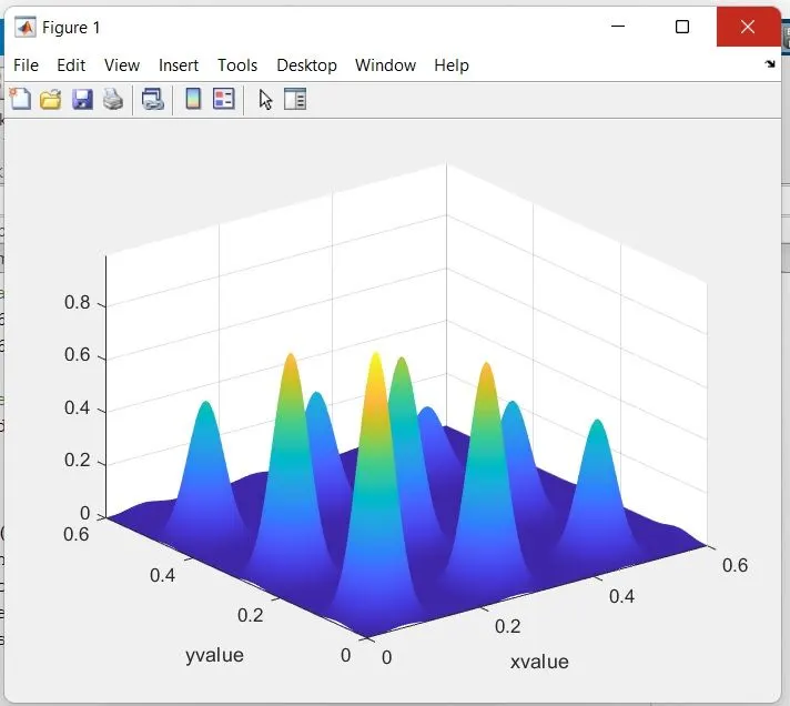
For finding minimum function by ga-

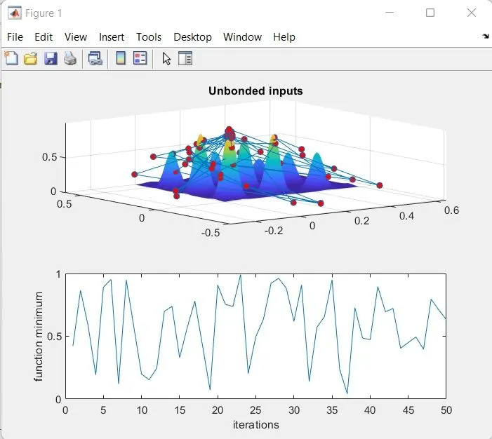
Study 1

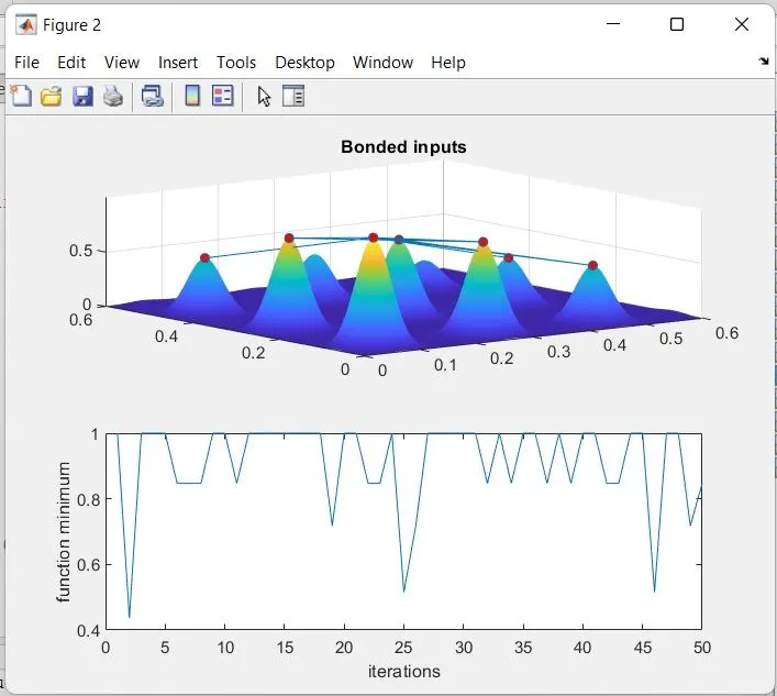
Study 2

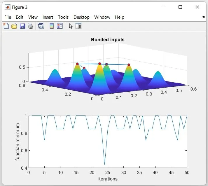
Study 3

Code expleation for 3 cases:

Study 1 statistical behaviour-

After creating x,y variable(input variable),
as it does not define the search space for ‘ga’, ‘ga’ does not know its actual space and the value for x,y go beyond or below to 0.6 or 0.

For that I use num_cases=50, means I am going to run it 50 times.

Sub-Step 1- I use ‘for loop’ and run the code from 1 to 50 times.
After that I call ga & use the new function which I created @stalagmite, pass 2 variable as input and store the output in GA_opt.
And than I store the value of ‘x &y’ in ‘xopt & yopt’

Sub-Step 2- Now to visualize my output, i use surface command(surfc), shading command(shading interp) is used to get smooth plot(without grid lines). in new figure window(figure1), I also use tic-toc command to calculate the time taken for evaluation. I use subplot command for multiple plotting,
1^st plot to show stalagmite function, and plotting the minimum value that ‘ga’ trying to predict, over 50 studies.
2^nd plot for showing the number of iteration at x-axis and during each iteration value changes which represents as Function maxima on y-axis.

Study 2 Statistical Behaviour(with upper & lower bound)-

In this study, I setup the bound condition for the variables x&y, as it is going above & below the 0 & 0.6.

By using syntax ‘ga’ I am giving x&y the upper limit and lower limit to 0 to 1. I a doing so, because in previous study, it was observed from the graph that the optimum output lies all over the graph, so make it more clear and optimum, I am applying the boundary condition.

Study 3 Increasing GA Iterations-
In addition with specifying bounds, I am also increasing initial population size. If population size is too small, we cannot find the global maxima, but we can find only local maxmia, which happens in study2.
Following the same procedure as in study-2, and increase the population size to 240 and applying the constraint ‘optimoptions’ and save its values in variable ‘options’ to allow the ga to predict the optimum solution from 240 population size.And plot graph for visual result