Week 4.1 - Genetic Algorithm
AIM
- Write a code in MATLAB to optimize the stalagmite function and find the global maxima of the function.
- Clearly explain the concept of genetic algorithm in your own words and also explain the syntax for ga in MATLAB in your report.
- Make sure that your code gives the same output, even if it is made to run several times.
- Plot graphs for all 3 studies and for F maximum vs no. of iterations. Title and axes labels are a must, legends could be shown if necessary.
Stalagmite
Stalagmite is a structure that is formed in caves by natural processes. It is an upward-growing mound of mineral deposits that have precipitated from water dripping onto the floor of a cave. Most stalagmites have rounded or flattened tips.
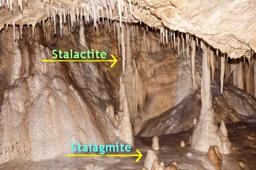
The stalagmite function is defined below:
GA (GENETIC ALGORITHM)
The genetic algorithm is a method for solving both constrained and unconstrained optimization problems that are based on natural selection, the process that drives biological evolution. The genetic algorithm repeatedly modifies a population of individual solutions. At each step, the genetic algorithm selects individuals at random from the current population to be parents and uses them to produce the children for the next generation. Over successive generations, the population "evolves" toward an optimal solution. You can apply the genetic algorithm to solve a variety of optimization problems that are not well suited for standard optimization algorithms, including problems in which the objective function is discontinuous, nondifferentiable, stochastic, or highly nonlinear. The genetic algorithm can address problems of mixed-integer programming, where some components are restricted to be integer-valued.
The genetic algorithm uses three main types of rules at each step to create the next generation from the current population:
-
Selection rules select the individuals, called parents, that contribute to the population at the next generation.
-
Crossover rules combine two parents to form children for the next generation.
-
Mutation rules apply random changes to individual parents to form children.
ga |
Find the minimum of a function using a genetic algorithm |
GA Syntax
min F(X) subject to: A*X <= B, Aeq*X = Beq (linear constraints)
X C(X) <= 0, Ceq(X) = 0 (nonlinear constraints)
LB <= X <= UB
X(i) integer, where i is in the index
vector INTCON (integer constraints)
Note: If INTCON is not empty, then no equality constraints are allowed.
That is:-
* Aeq and Beq must be empty
* Ceq returned from NONLCON must be empty
X = ga(FITNESSFCN,NVARS) finds a local unconstrained minimum X to the
FITNESSFCN using ga. NVARS is the dimension (number of design variables) of the FITNESSFCN. FITNESSFCN accepts a vector X of size
1-by-NVARS, and returns a scalar evaluated at X.
X = ga(FITNESSFCN,NVARS,A,b) finds a local minimum X to the function
FITNESSFCN, subject to the linear inequalities A*X <= B. Linear
constraints are not satisfied when the PopulationType option is set to
'bitString' or 'custom'.
X = ga(FITNESSFCN,NVARS,A,b,Aeq,beq) finds a local minimum X to the
function FITNESSFCN, subject to the linear equalities Aeq*X = beq as
well as A*X <= B. (Set A=[] and B=[] if no inequalities exist.) Linear
constraints are not satisfied when the PopulationType option is set to
'bitString' or 'custom'.
X = ga(FITNESSFCN,NVARS,A,b,Aeq,beq,lb,ub) defines a set of lower and
upper bounds on the design variables, X, so that a solution is found in
the range lb <= X <= ub. Use empty matrices for lb and ub if no bounds
exist. Set lb(i) = -Inf if X(i) is unbounded below; set ub(i) = Inf if
X(i) is unbounded above. Linear constraints are not satisfied when the
PopulationType option is set to 'bitString' or 'custom'.
X = ga(FITNESSFCN,NVARS,A,b,Aeq,beq,lb,ub,NONLCON) subjects the
minimization to the constraints defined in NONLCON. The function
NONLCON accepts X and returns the vectors C and Ceq, representing the
nonlinear inequalities and equalities respectively. ga minimizes
FITNESSFCN such that C(X)<=0 and Ceq(X)=0. (Set lb=[] and/or ub=[] if
no bounds exist.) Nonlinear constraints are not satisfied when the
PopulationType option is set to 'bitString' or 'custom'.
X = ga(FITNESSFCN,NVARS,A,b,Aeq,beq,lb,ub,NONLCON,options) minimizes
with the default optimization parameters replaced by values in OPTIONS.
OPTIONS can be created with the OPTIMOPTIONS function.
X = ga(FITNESSFCN,NVARS,A,b,[],[],lb,ub,NONLCON,INTCON) requires that
the variables listed in INTCON take integer values. Note that ga does
not solve problems with integer and equality constraints. Pass empty
matrices for the Aeq and beq inputs if INTCON is not empty.
X = ga(FITNESSFCN,NVARS,A,b,[],[],lb,ub,NONLCON,INTCON,options)
minimizes with integer constraints and the default optimization
parameters replaced by values in OPTIONS. OPTIONS can be created with
the OPTIMOPTIONS function.
Need to find the global maxima of the study area.
%stalagmite funtion code

function [f] = stalagmite(input_vector);

%inputs

x = input_vector(1);
y = input_vector(2);

%calculation of f1,f2,f3,f4

f1 = sin(5.1*pi*x + 0.5).^6;
f2= sin(5.1*pi*y + 0.5).^6;
u= -4*log(2);
v =(x - 0.0667).^2/0.64;
w = (y - 0.0667).^2/0.64;
f3 = exp(u*v);
f4 = exp(u*w);

%result

f= -(f1*f2*f3*f4);
end
2. Program Code
clear all
close all
clc

%inputs

x = linspace(0,0.6,150);
y = linspace(0,0.6,150);

%number of iteration
iteration = 50;

%meshgrid of x and y
[xx yy] = meshgrid(x,y);

%to find the value of 'f'

for i = 1:length(xx);

    for j = 1:length(yy);

        input_vector(1)= xx(i,j);
        input_vector(2)= yy(i,j);
        f(i,j) = stalagmite(input_vector);


    end
end

%Study 1
%unbounded case
tic %timer on

for i = 1:iteration;

[result,fopt(i)] = ga(@stalagmite,2);
xopt(i) = result(1);
yopt(i) = result(2);
end

study_time_1 = toc %timer off

%plotting study 1
figure(1)
subplot(2,1,1)
surf(x,y,-f)
title('Study 1 - Unbounded')
shading interp
hold on
plot3(xopt,yopt,-fopt,'marker','o')
subplot(2,1,2)
plot(-fopt)
xlabel('Iteration')
ylabel('Function Maximum')


%Study 2
%bounded case

tic %timer on

for i=1:iteration;
    [result,fopt2(i)]=ga(@stalagmite,2,[],[],[],[],[0;0],[0.6;0.6]);
    xopt(i)=result(1);
    yopt(i)=result(2);
end
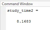
study_time2=toc  %timer off

%plotting - study 2
figure(2)
subplot(2,1,1)
surf(x,y,-f)
title('Study 2 - Bounded')
shading interp
hold on
plot3(xopt,yopt,-fopt2,'marker','o')
subplot(2,1,2)
plot(-fopt2)
xlabel('Iteration')
ylabel('Funtion Maximum')


%study 3
%bounded, increased iteration, population change

tic %timer on

options=optimoptions('ga')
options=optimoptions(options,'populationsize',300)

%increased iteration
iteration_inc = 300;

for i=1:iteration_inc
    [results,fopt(i)]=ga(@stalagmite,2,[],[],[],[],[0;0],[0.1;0.1],[],[],options);
    xopt(i)=results(1);
    yopt(i)=results(2);
end
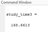
study_time3=toc %timer off

%plotting - Study 3

figure(3)
subplot(2,1,1)
surf(x,y,-f)
title('Study 3 - Bounded, Increased Iteration, Population change')
shading interp
hold on
plot3(xopt,yopt,-fopt,'marker','o')
subplot(2,1,2)
plot(-fopt)
xlabel('Iteration')
ylabel('Function Maximum')

%position of maximum funtion value
coordinate = [results]
Explanation:
Stalagmite function code explanation:
Stalagmite function code gives the height of the stalagmite for the respective x-axis and y-axis.
Initially, the function is defined. Then the inputs are called.
Calculation of 'f' - the height of stalagmites are calculated.
While saving the value of 'f' we multiply with (-1) in order to get a negative value as we use ga function to the global maxima result.
[ ga -Finds the minimum of a function using a genetic algorithm]
Program code explanation:
In this, we study three methods and conditions to find the global maxima using the ga.
First, getting the initial values of "x" and "y".
x = linspace(0,0.6,150);
y = linspace(0,0.6,150);
then, the number of iteration
iteration = 50;
using the meshgrid to get "xx" and "yy"
[xx yy] = meshgrid(x,y);
then, finding the value of "f" using stalagmite funtion code
for i = 1:length(xx);
for j = 1:length(yy);
input_vector(1)= xx(i,j);
input_vector(2)= yy(i,j);
f(i,j) = stalagmite(input_vector);
end
end
firstly, study 1- Unbounded case( no conditions )
using the ga to find the minima ( as we multiplied -1 with the result in stalagmite function code, output will be correct while using ga)
using timer to know the study time.
for i = 1:iteration;
[result,fopt(i)] = ga(@stalagmite,2);
xopt(i) = result(1);
yopt(i) = result(2);
end
then, plotting the study case 1 to get the required output.
Using subplot option to get two plots in same figure
figure(1)
subplot(2,1,1)
surf(x,y,-f)
title('Study 1 - Unbounded')
shading interp - to get a smooth curve
hold on
plot3(xopt,yopt,-fopt,'marker','o') - to get the markings for the results that are got.
subplot(2,1,2) - second plot
plot(-fopt) - plotting the value of "fopt"
Labelling the axes
xlabel('Iteration')
ylabel('Function Maximum')
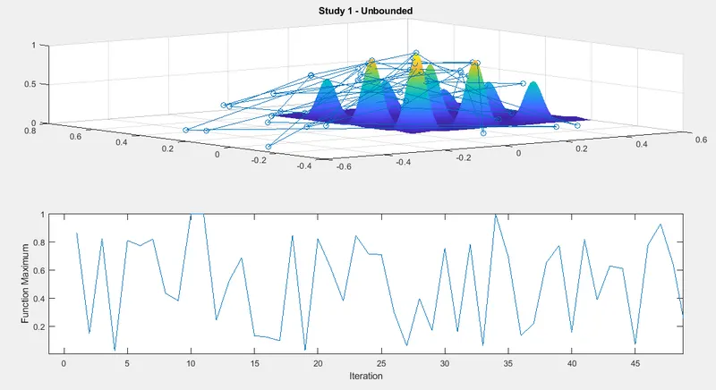
StudyCase - 1 Results
This graph gives us information about the peaks. but the result is varying from iteration to iteration as the case is unbounded and no conditions given.
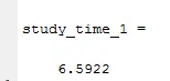
Study time for case 1 is 6.5922 sec
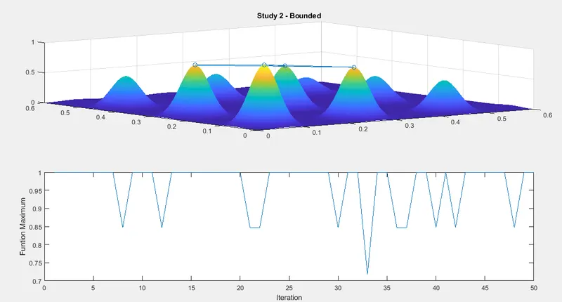
Study 2 - Bounded case
Almost similar, to that of the Unbound case but here we give the boundary conditions as ga doesn't know the boundaries of "x" and "y"
using the ga to find the minima ( as we multiplied -1 with the result in stalagmite function code, the output will be correct while using ga)
[result,fopt2(i)]=ga(@stalagmite,2,[],[],[],[],[0;0],[0.6;0.6]);
Syntax
[X,FVAL]= ga(FITNESSFCN,NVARS,A,b,Aeq,beq,lb,ub) defines a set of lower and
upper bounds on the design variables, X, so that a solution is found in
the range lb <= X <= ub. Use empty matrices for lb and ub if no bounds
exist. Set lb(i) = -Inf if X(i) is unbounded below; set ub(i) = Inf if
X(i) is unbounded above. Linear constraints are not satisfied when the
PopulationType option is set to 'bitString' or 'custom
lower bound = 0;0
upper bound = 0.6;0.6
so that a solution is found in
the range lb <= X <= ub.
then, Plotting Study Case 2
StudyCase - 2 Results (Bounded case)
Study time for case 2 is 8.16833 sec
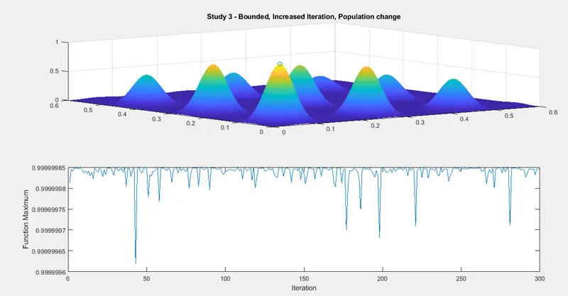
Study 3 - Bounded, increased iteration, population change
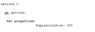
In this case, we use options of ga and change the population to 300
options=optimoptions('ga')
options=optimoptions(options,'populationsize',300)
increase in iterations
iteration_inc = 300;
Also, changing the Boundary of search lb = 0;0 & ub = 0.1;0.1
timer is used to know the study time
for i=1:iteration_inc
[results,fopt(i)]=ga(@stalagmite,2,[],[],[],[],[0;0],[0.1;0.1],[],[],options);
xopt(i)=results(1);
yopt(i)=results(2);
end
Then, Plotting of the study case 3
StudyCase - 3 Results (Bounded, increased iteration, population change)
Study time for case 3 is 168.6613 sec
When comparing the results of all three study, study 3 gives accurate and a single result stating the highest or global maxima is 0.99999985 , but this study takes time as the number of iteration has been increased and population size is also varied.
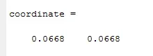
To get the position of maximum function value
coordinate = [results]
coordinate at which there is global maxima value:
References,
https://in.mathworks.com/help/gads/genetic-algorithm.html?s_tid=CRUX_lftnav
https://in.mathworks.com/help/gads/ga.html?s_tid=doc_ta
Thanks,
Vishal