Project 2 - Rankine cycle Simulator

AIM:-

• To create a Rankine Cycle Simulator
• Calculate the state points of the Rankine Cycle.
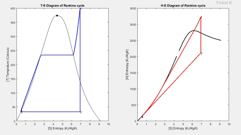
• Plot the T-S and H-S plots.
• Required Inputs:

Turbine Inlet temperature = 400° C

Turbine Inlet Pressure = 30 bars

Turbine Outlet Pressure = 0.05 bars = Condenser Inlet Pressure

Calculate the followings,

1. Net Work ratio

2. Back Work ratio

RANKINE CYCLE

A steam power plant works on the principle of the Rankine cycle and hence we can say that a steam power plant will be designed in such a way that the process of each component of the power plant will follow the process of the Rankine cycle.

The theoretical Rankine cycle or ideal Rankine cycle comprises of,

Process 1-2 = Turbine ( Reversible Adiabatic Process/ Isentropic Proces)

Process 2-3 = Condenser ( Constant Pressure Process/ Isobaric Process)

Process 3-4 = Pump ( Reversible Adiabatic Process/ Isentropic Process)

Process 4-1= Boiler( Constant Pressure Process/ Isobaric Process)

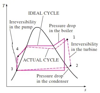
Processes of an actual Rankine cycle will be slightly different from the processes of an ideal Rankine cycle because in practice there will be various irreversibilities in various components of the Rankine cycle. Heat losses to surrounding and friction will be the main causes of irreversibilities and we will also discuss here the deviation of the actual vapour cycle with the ideal Rankine cycle.

Diagram of ideal Rankine cycle

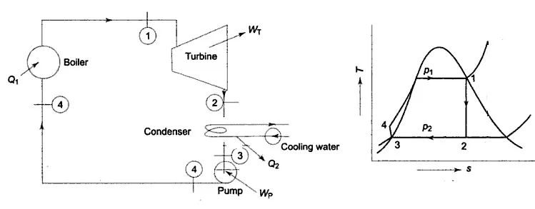
Ideal Rankine cycle vs Actual Rankine cycle

The actual Rankine cycle will have irreversibilities in various components of the Rankine cycle in order to get higher performance and to increase the stability of the cycle.

PROCEDURE

1.We will use the standard Xsteam library to get the steam table data for water.

2. Get inputs from the user

Pressure at the turbine inlet [Bar]

The temperature at the turbine inlet [Celcius]

Pressure at the Condenser[Bar]

4. Calculate state variables.

5. Calculate the turbine work and pump work, Efficiency, SSC(Specific Steam Consumption)

6. Plot the T-S and H-S plots.

7. print all the performance and outputs needed.

inputs from the user

Pressure at the turbine inlet [Bar] 30

The temperature at the turbine inlet [Celcius] 400

Pressure at the Condenser[Bar] 0.05

PROGRAM

MATLAB CODE FOR RANKINE CYCLE

% Rankine Cycle
 
%program start 
% Clearing workspace, command window & closing all
clear all
close all
clc
 
% Step 1
% Print discription of all process
fprintf(' RANKINE CYCLE SIMULATOR');
fprintf('\n');
fprintf('\n');
fprintf('1-2  Isentropic Expansion in the Turbine');
fprintf('\n');
fprintf('2-3  Constant Pressure Heat Rejection by the Condenser')
fprintf('\n');
fprintf('3-2  Isentropic Compression in the Pump')
fprintf('\n');
fprintf('4-1  Constant Pressure Heat Addition by the Boiler')
fprintf('\n');
fprintf('\n');
 
% Step 2
% Taking all inputs arguments
P1 = input('Enter the Pressure at the Turbine Inlet (in bar): ');
fprintf('\n');
T1 = input('Enter the Temperature at the Turbine inlet (in Degree celsius): ');
fprintf('\n');
P2 = input('Enter the Pressure at the Condenser (in bar): ');
fprintf('\n');
 
% Step 3 
%finding and getting all values and calculating 
% Pressures at all points
P4 = P1;
P3 = P2;
 
% entropy
S1 = XSteam('s_pT',P1,T1); 
S2 = S1; % entropy at point 1 is equal to entropy at point 2
Sf2 = XSteam('sL_p',P2);
Sg2 = XSteam('sV_p',P2);
Sfg2 = Sg2 - Sf2;
 
% X = dryness fraction % We know that S2 = Sf2 + X(Sfg2)
X= (S2-Sf2)/Sfg2 ;
 
% Enthalpy 
H1 = XSteam('h_pT',P1,T1); 
Hf2 = XSteam('hL_p',P2); 
Hg2 = XSteam('hV_p',P2);
Hfg2 = Hg2 - Hf2;
H2 = Hf2 + X*Hfg2;
 
H3 = Hf2; % enthalpy state point 3
 
if (X > 1) %if dryness fraction X>1,
    T2 = XSteam('T_ps',P2,S2);
    T3 = XSteam('Tsat_p',P2);
 
    Td = linspace(T2,T3,50);
 
    S_2 = XSteam('sV_T',T3);
    S3 = XSteam('sL_T',T3);
 
    S4 = S3; % ( 3-4 isentropic process) so, S3 = S4
 
else %else dryness fraction X<1,
    T2 = XSteam('Tsat_p',P2);
    T3 = T2;   
    S3 = Sf2; % State pont 3
    S4 = S3; % ( 3-4 isentropic process) so, S3 = S4
end
 
V3 = XSteam('vL_p',P3); %specific volume
H4 = V3*(P1-P2)*100  + H3; % enthalpy at state point 4
Cp = XSteam('Cp_ps',P3,S3); 
Cv = XSteam('Cv_ps',P3,S3);
G = Cp/Cv  ;  %gamma 
Y = (G-1)/G;  % let Y be (gamma-1) /gamma ; which we will use for calculating T4 
T4 = T3*((P4/P3)^Y); % Temperature at point 4
T5 = XSteam('Tsat_p',P1);
T6 = T5; 
S5 = XSteam('sL_T',T5);
S6 = XSteam('sV_T',T6);
 
% Step 4
%Calculation
% Turbine work
W_T = H1 - H2;
% Pump work
W_P = H4 - H3;
% Net work, Back work ratio,SSC and thermal efficiency of Rankine cycle
W_net = W_T-W_P;
Backwork_ratio = W_P/W_T; 
SSC = 3600/W_net; %specific steam consumption
Qin = H1 - H4; %heat input
Efficiency = (W_net/Qin)*100;
 
% Step 5
%printing all values at different state point 
fprintf('RESULTS');
fprintf('\n');
fprintf('\n');
 
% state point 1
fprintf('State point-1');
fprintf('\n');
 
fprintf('P1 = %f Bar',P1);
fprintf('\n');
 
fprintf('T1 = %f Celsius',T1);
fprintf('\n');
 
fprintf('S1 = %f kJ/kgK',S1);
fprintf('\n');
 
fprintf('H1 = %f kJ/kgK',H1');
fprintf('\n');
fprintf('\n');
 
% state point 2 
fprintf('State point-2');
fprintf('\n');
 
fprintf('P2 = %f Bar',P2);
fprintf('\n');
 
fprintf('T2 = %f Celsius',T2);
fprintf('\n');
 
fprintf('S2 = %f kJ/kgK',S2);
fprintf('\n');
 
fprintf('H2 = %f kJ/kgK',H2');
fprintf('\n');
 
fprintf('X(dryness fraction) = %f',X);
fprintf('\n');
fprintf('\n');
 
% state point 3 
fprintf('State point-3');
fprintf('\n');
 
fprintf('P3 = %f Bar',P3);
fprintf('\n');
 
fprintf('T3 = %f Celsius',T3);
fprintf('\n');
 
fprintf('S3 = %f kJ/kgK',S3);
fprintf('\n');
 
fprintf('H3 = %f kJ/kgK',H3);
fprintf('\n');
fprintf('\n');
 
% state point 4 
fprintf('State point-4');
fprintf('\n');
 
fprintf('P4 = %f Bar',P4);
fprintf('\n');
 
fprintf('T4 = %f Celsius',T4);
fprintf('\n');
 
fprintf('S4 = %f kJ/kgK',S4);
fprintf('\n');
 
fprintf('H4 = %f kJ/kgK',H4');
fprintf('\n');
fprintf('\n');
 
% Step 6
%plotting of the graph
 
% Data - boiler sensible heat addition at superheated condition
T = linspace(T6,T1,500);
for i = 1:length(T)
    S(i) = XSteam('s_pT',P1,T(i));
    H(i) = XSteam('h_pT',P1,T(i));
end
 
% Data - saturation temperature curve 
maxt = linspace(1,T1,500);
for j = 1:length(maxt)
    satlS(j) = XSteam('sL_T',maxt(j));
    satvS(j) = XSteam('sV_T',maxt(j));
    satlH(j) = XSteam('hL_T',maxt(j));
    satvH(j) = XSteam('hV_T',maxt(j));
end
 
%T-S Diagram for Rankine cycle
subplot(1,2,1)
% plot - saturation curves
plot(satlS,maxt,'color','k')% saturation liquid temperatures
hold on
plot(satvS,maxt,'color','k')% saturation vapour temperatures
plot(4.4230,373.6,'o','MarkerFaceColor','k','MarkerSize',7) % critical temperature
 
%plot - Curve for points t5 and t6
line([S5 S6],[T5 T6],'Color','b','lineWidth',2)
%plot - Curve for points t6 and T1
plot(S,T,'Color','b','lineWidth',2)
%plot - Curve for points T1 and T2
line([S1 S2],[T1 T2],'Color','b','lineWidth',2)
 
if (X > 1)   
    % Data - constant pressure curve at boiler inlet if present
    for i = 1:length(Td)
    Sd(i) = XSteam('s_pT',P2,Td(i));
    Hd(i) = XSteam('h_pT',P2,Td(i));
    end
 
%plot - Curve for points T2 and t_2 (if present)     
plot(Sd,Td,'color','b','lineWidth',2)
% plot - line for t_2 and T3 (if present)
line([S_2 S3],[T3 T3],'Color','b','lineWidth',2)
else
    line([S2 S3],[T2 T3],'color','b','lineWidth',2) 
end
 
%plot - Curve for points T3 and T4
line([S3 S4],[T3 T4],'Color','b','lineWidth',2)
 
% plot - Constant pressure heat addition curve till saturation liquid line
line([S4 S5],[T4 T5],'Color','b','lineWidth',2)
 
% labelling of graph
title('T-S Diagram of Rankine cycle')
xlabel('[S] Entropy (KJ/KgK)')
ylabel('[T] Temprature (Celcius)')
 
% Marking the state points
text(S1,T1,"1");
text(S2,T2,"2");
 
if (X > 1)
    text(S_2,T3,"2'");
end
text(S3,T3,"3");
text(S4,T4,"4");
 
%H-S diagram for rankine cycle
subplot(1,2,2)
% plot for saturation curves of liquid and vapuor
plot(satlS,satlH,'color','k','lineWidth',2)
hold on
plot(satvS,satvH,'color','k','lineWidth',2)
 
% plot - isentropic expansion line
line([S1 S2],[H1 H2],'color','r','lineWidth',2)
 
 
if (X > 1)
    
    H_2 = XSteam('h_ps',P2,S_2);
    %plot - constant pressure heat addition ,if outlet steam is superheatedcond.
    plot(Sd,Hd,'color','r','lineWidth',2)
    
    % Data - constant pressure heat rejection curve enthalpy values
    entropy = linspace(S_2,S3,100);
    for k = 1:length(entropy);
        enthlpy(k) = XSteam('h_ps',P2,entropy(k));
    end
    
    % Plot - constant pressure heat rejection curve 
    plot(entropy,enthlpy,'color','r','lineWidth',2)
else
    
    % Data - constant pressure heat rejection curve enthalpy values if
    % steam is wet or dry saturated vapour
    entropy = linspace(S2,S3,100);
    for k = 1:length(entropy);
        enthlpy(k) = XSteam('h_ps',P2,entropy(k));
    end
    
     % Plot - constant pressure heat rejection curve 
    plot(entropy,enthlpy,'color','r','lineWidth',2)
end
 
%plot - Isentropic compression line
line([S3 S4],[H3 H4],'color','r','lineWidth',2)
 
% data - Constant pressure heat addition curve enthalpy values
entrpy1 = linspace(S4,S1,100);
for l = 1:length(entrpy1)
    enthlpy1(l) = XSteam('h_ps',P1,entrpy1(l));
end
 
% plot - Constant pressure heat addition curve 
plot(entrpy1,enthlpy1,'color','r','lineWidth',2)
 
% labelling of graph
title('H-S Diagram of Rankine cycle')
xlabel('[S] Entropy (KJ/KgK)')
ylabel('[H] Enthalpy (KJ/KgK)')
 
% Marking the state points
text(S1,H1,"1");
text(S2,H2,"2");
 
if (X > 1)
    text(S_2,H_2,"2'");
end
text(S3,H3,"3");
text(S4,H4,"4");
 
% Step 7
% Performance parameters of Rankine cycle
 
fprintf('Performance of Rankine cycle');
fprintf('\n');
fprintf('\n');
fprintf('Turbine work = %f kJ/kg',W_T);
fprintf('\n');
fprintf('Pump work = %f kJ/kg',W_P);
fprintf('\n');
fprintf('Back Work ration = %f',Backwork_ratio);
fprintf('\n');
fprintf('Thermal efficiency = %f %%',Efficiency);
fprintf('\n');
fprintf('Specific Steam Consumption = %f kg/kWh',SSC);
fprintf('\n');
 
%program end

CODE EXPLANATION

Before starting the code save the XSteam function code

Starting with comment Rankine cycle,

then close all; clear all and clc command for Clearing workspace, command window & closing all

Step 1:

Printing the heading and description of all the processes

Step 2:

Taking the input arguments from the user

P1[Turbine input pressure]

T1[Temperature at Turbine input]

P2[Turbine outlet pressure]

Step 3

finding and getting all values and calculating them

Pressures at all points

P4 = P1 & P3 = P2 [isobaric processes]

getting the values of entropy using the XSteam table

S1 = XSteam('s_pT',P1,T1)

S2 = S1 [entropy at point 1 is equal to entropy at point 2] Isentropic process

Sf2 = XSteam('sL_p',P2) Entopy at Fluid state

Sg2 = XSteam('sV_p',P2) Entopy at vapour state

Sfg2 = Sg2 - Sf2 [Getting the difference between Entropy at vapor state abdEntopy at Fluid state]

then, calculating dryness fraction 'X' [ We know that S2 = Sf2 + X(Sfg2) ] hence,

X= (S2-Sf2)/Sfg2

Getting the Enthalpy values

H1 = XSteam('h_pT',P1,T1)

Hf2 = XSteam('hL_p',P2) Enthalpy at fluid[liquid] state at lower Pressure P2

Hg2 = XSteam('hV_p',P2) Enthalpy at vapour[gas] state at lowe Pressure P2

Hfg2 = Hg2 - Hf2 [Getting the difference]

H2 = Hf2 + X*Hfg2 calculating the Value of Enthalpy at point 2

H3 = Hf2; [enthalpy state point 3]

Using if condition for two different types of dryness fraction [X>1] and else condition

then, getting the values of Entropy and Temperature according to the condition

in the next step, we find

V3 = XSteam('vL_p',P3); [specific volume]

H4 = V3*(P1-P2)*100 + H3; [ enthalpy at state point 4]

Cp = XSteam('Cp_ps',P3,S3) Specific heat at constant pressure

Cv = XSteam('Cv_ps',P3,S3) Specific heat at constant volume

G = Cp/Cv ; [gamma]

Y = (G-1)/G; [ let Y be (gamma-1) /gamma ; which we will use for calculating T4]

using adiabatic process formulae

T4 = T3*((P4/P3)^Y); Temperature at point 4

Getting the other values at differnt points which we use for plotting

T5 = XSteam('Tsat_p',P1)

T6 = T5

S5 = XSteam('sL_T',T5)

S6 = XSteam('sV_T',T6)

Step 4

Calculation in Rankine cycle

W_T = H1 - H2 work done by Turbine Pump work

W_P = H4 - H3 work done by Pump

W_net = W_T-W_P [Net work done ]

Backwork_ratio = W_P/W_T [ Back work ratio]

SSC = 3600/W_net [specific steam consumption]

Qin = H1 - H4; [heat input]

Efficiency = (W_net/Qin)*100 [thermal efficiency of Rankine cycle]

Step 5

printing all values at different state point

Step 6

plotting of the graph

Starting with the Temperature vs Entropy graph

drawing the vapor and gas saturation lines

then, plotting the Rankine cycle process

labeling the axis; marking the points; Title giving

similarly, doing the same for the Enthalpy vs Entropy graph

Step 7

Printing the Performance parameters of the Rankine cycle and ending the program.

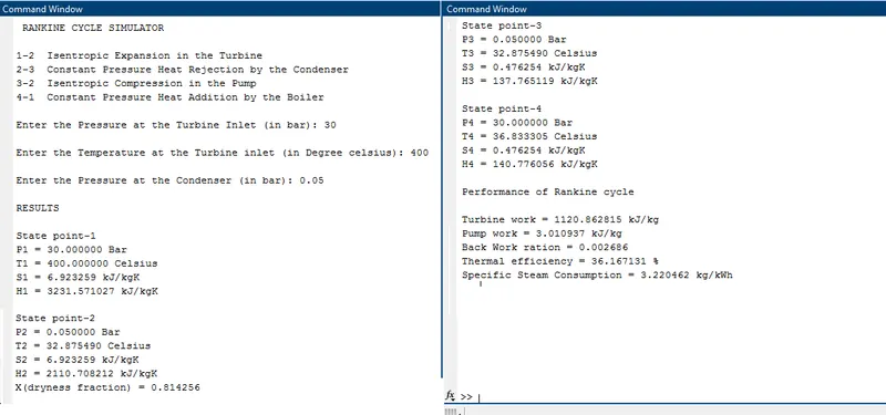
OUTPUT

After running and giving inputs to the program we get,

(i)Graph window

(ii)Command Window

CONCLUSION

The Rankine cycle is widely used in many mechanical cycles like thermal power plants, energy generation cycles, etc. So making it handy and quick, saves a lot of time.

Thanks,

Vishal R