Project 2 - Rankine cycle Simulator
AIM: Create a Rankine Cycle Simuator using MATLAB.
OBJECTIVES:
- Write a code to Calculate the state points in Rankine Cycle based on the user inputs.
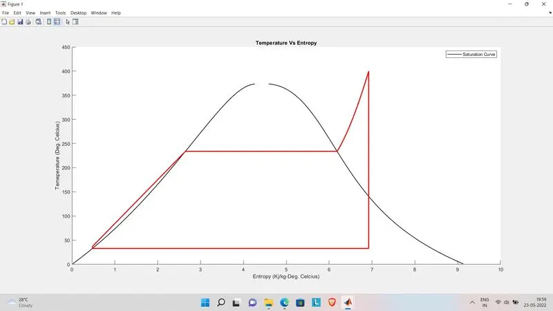
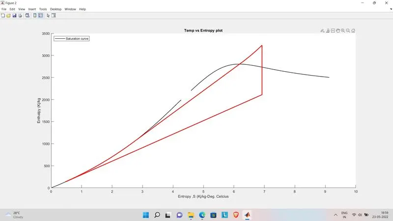
- plot the T-S and H_S diagram
- Explain the working of the Rankine Cycle
THEORY:
The Rankine cycle is an idealized thermodynamic cycle that converts heat into mechanical work while undergoing a phase change. It is an idealized cycle in which friction losses in each of the four components are neglected. The heat is supplied externally to a closed loop, which usually uses water as the working fluid. The working fluid is continuously evapourated and condensed.
Components of a Rankine Cycle:
- Boiler
- Turbine
- Condenser
- Pump
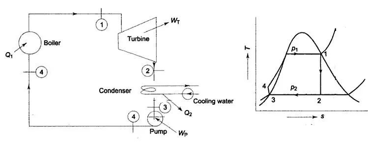
Processess in the Rankine Cycle
1-2: Isentropic Expansion in the Turbine: Vapor from the boiler outlet enters the turbine at state 2, where it expands isentropically over the turbine fixed and moving blade to produce work done in the form of mechanical rotation of the turbine shaft, which is connected to the electrical generator.
Work delivered by the turbine (Neglecting heat transfer with the surroundings)
Wturbine out= h1-h2
2-3: Constant Pressure Heat Rejection in the Condenser: At state-2, vapor enters the condenser. The change of phase occurs as vapor is condensed to liquid at constant-pressure in the condenser by transferring the steam’s heat to the circulating water flow through the tubes of the condenser. Change of phase occurs in the condenser, and the working fluid leaving the condenser is in a liquid state and marked as point 3.
Energy rejected in the condenser.
qout= h2-h3
3-4: Isentropic Compression in the pump: Water exits the condenser at state 3 and enters the pump. This pump raises the pressure of the water by imparting work during the processes. In units of smaller size and low specific volume, this small work can be neglected compared to the work-output of a steam turbine.
Work was done on the pump per kg of water,
W43= h4-h3.
4-1: Constant Pressure Heat addition on Boiler: The boiler is a large heat exchanger where heat liberating fuel like coal, lignite, or oil transfers the heat indirectly to water at constant pressure. Water enters the steam boiler from the boiler feed pump as a compressed liquid at state-1 and is heated to the saturation temperature as shown in the T-s diagram as state-3.The energy balance in the boiler is or energy added in a steam generator,
qin= h1-h4
CODE:
% Rankine Cycle Simulator
clear all
close all
clc

%Input the initial condition for Calculation of State points
p1 =input("\n Inlet Pressure in Turbine (bar)= ");
t1 =input("\n Inlet Temperature in the Turbine (in degree C)= ");
p2 =input("\n Condenser Inlet Pressure (bar)= ");

%Extracting data from Xsteam file for each state points
% for State point 1
h1= XSteam('h_pT', p1,t1);      % Enthalpy at pressure and temperature 1
s1= XSteam('s_pT',p1,t1);       % Entropy at pressure and temperature 1

% for State point 2
s2=s1;                          % Isentropic Expansion
sf2= XSteam('sL_p',p2);         % Saturated Liquid Entropy at pressure
sg2= XSteam('sV_p',p2);         % Saturated Vapour Entropy at pressure
sfg= sg2-sf2;
x2= (s2-sf2)/sfg;               % Dryness fraction at state point 2
hf2= XSteam('hL_p',p2);         % Saturated Liuid Enthalpy at pressure
hg2= XSteam('hV_p',p2);         % Saturated Vapour Enthalpy at pressure
h2= hf2 + (x2*(hg2-hf2));            % Enthalpy at state point 2

% For State point 3
p3=p2;                          % Constant pressure Heat Rejection
s3= XSteam('sL_p', p3);         % Saturated Liquid Entropy at pressure
h3= XSteam('hL_p',p3);          % Saturated Vapour Entroy at pressure

% For State point 4
s4=s3;                          % Isentropic Compression
p4=p1;                          % Constant pressure heat addition


% Work Done by Turbine(W_T)
W_T= h1-h2;

% Work done by the pump(W_P)
v3= XSteam('vL_p',p3);          %Volume at state point 3
W_P = v3*(p4-p3);
h4= h3+W_P;                     % Enthalpy at state point 4

% Net Workdone (W_net)
W_net= W_T-W_P;

% Heat into the System
Q_in= h1-h4;

% Heat out of the System
Q_out= h2-h3;

% Thermal Efficiency of the Cycle
eff= (W_net/Q_in)*100;


% Calculating the Back Work Ratio
BW= W_P/W_T;

% Calculation of the Specific Steam Consumption
% Specific Steam Consumption= Mass flow rate/ Net Work Done
SSC= 3600/W_net;

% Calculation of the Temperatures at state point 2,3,4

t3 = XSteam('Tsat_p',p3);           % Saturation Temperature at Pressure 3
t2 = t3;                            % Becuase of Constant Pressure Heat addition
Cp4 = XSteam('Cp_ps',p4,s4);        % Specific isobaric heat capacity
Cv4 = XSteam('Cv_ps',p4,s4);        % Specific isochoric heat capacity
k = Cp4/Cv4;
t4 = t3/((p3/p4)^((k-1)/k));        % Temperature at State point 4
t6 = XSteam('Tsat_p', p1);          % Saturated Temperature at Pressure 1
s5 = XSteam('sL_p', p1);            % Saturated Liquid entropy at pressure 1
s6 = XSteam('sV_p', p1);            % Saturated Vapour entropy at Pressure 1
h5 = XSteam('hL_p', p1);            % Saturated Liquid Enthalpy at Pressure 1
h6 = XSteam('hV_p', p1);            % Saturated Vapour Enthalpy at pressure 1
t5 = t6;

%Plotting for Saturation Line
T = linspace(1,600,1000);
for i = 1:length(T)
    sf(i) = XSteam('sL_T' ,T(i));   % Saturated Liquid Entropy
    sg(i) = XSteam('sV_T' ,T(i));   % Saturated Vapour Entropy
    hf(i) = XSteam('hL_T' ,T(i));   % Saturated Liquid Enthalpy
    hg(i) = XSteam('hV_T' ,T(i));   % Saturated Vapour Enthalpy

end

% Plotting T-S Diagram for Rankine Cycle
figure(1)
hold on
plot(sf,T,'color','black','linewidth',1)   % Plotting of the Saturation Liquid Curve
plot(sg,T,'color','black','linewidth',1)   % Plotting of the Saturation Vapour Curve

plot([s1 s2],[t1 t2], 'color', 'r', 'linewidth',2)
plot([s2 s3],[t2 t3], 'color', 'r', 'linewidth',2)
plot([s3 s4],[t3 t4], 'color', 'r', 'linewidth',2)
plot([s4 s5],[t4 t5], 'color', 'r', 'linewidth',2)
plot([s5 s6],[t5 t6], 'color', 'r', 'linewidth',2)

s_1 = linspace(s1,s6,1000);
for j = 1:length(s_1)
    Tc(j) = XSteam('T_ps',p1,s_1(j));
end
plot(s_1,Tc,'color','r','linewidth',2)

title('Temperature Vs Entropy')
xlabel('Entropy (Kj/kg-Deg. Celcius)')
ylabel('Temeperature (Deg. Celcius)')
legend('Saturation Curve','Location','northeast')

% Plotting H-S Diagram for Rankine Cycle
figure(2)
hold on
plot(sf,hf,'color','black','linewidth',1)  % Plotting of the Saturation Liquid Curve
plot(sg,hg,'color','black','linewidth',1)  % Plotting of the Satuartion Vapour Curve

plot([s1 s2],[h1 h2],'color','r','linewidth',2)
plot([s2 s3],[h2 h3],'color','r','linewidth',2)
plot([s3 s4],[h3 h4],'color','r','linewidth',2)
hc = linspace(h4,h5,1000);
for k = 1:length(hc)
    s_c(k) = XSteam('s_ph',p1,hc(k));
end
plot(s_c,hc,'color','r','linewidth',2)
plot([s5 s6],[h5 h6],'color','r','linewidth',2)
for l = 1:length(s_1)
    h_c(l) = XSteam('h_ps',p1,s_1(l));
end
plot(s_1,h_c,'color','r','linewidth',2)

title('Temp vs Entropy plot')
xlabel('Entropy ,S (Kj/kg-Deg. Celcius')
ylabel('Enthalpy (Kj/kg')
legend('Saturation curve','location','northwest')


% Displaying the Rankine Cycle processes
fprintf("\n\n*************RANKINE CYCLE***************\n\n");
disp("1-2 is the Isentropic Expansion in Turbine");
disp("2-3 is the Constant pressure Heat Rejection in Condenser");
disp("3-4 is the Isentropic Compression in Pump ");
fprintf("4-1 is the Constant pressure Heat Addition in Boiler\n\n");

%Displaying Results in the command window
fprintf("\n\n***************RESULTS***************\n\n")
fprintf("At State point 1\n");
fprintf("P1= %8f bar\n",p1);
fprintf("T1= %8f in Deg. Celcius\n",t1);
fprintf("H1= %8f KJ/kg\n",h1);
fprintf("S1= %8f KJ/kg-Deg. Celcius\n\n",s1);

fprintf("At State point 2\n");
fprintf("P2= %8f bar\n",p2);
fprintf("T2= %8f in Deg. Celcius\n",t2);
fprintf("H2= %8f KJ/kg\n",h2);
fprintf("S2= %8f KJ/kg-Deg. Celcius\n\n",s2);

fprintf("At State point 3\n");
fprintf("P3= %8f bar\n",p3);
fprintf("T3= %8f in Deg. Celcius\n",t3);
fprintf("H3= %8f KJ/kg\n",h3);
fprintf("S3= %8f KJ/kg-Deg. Celcius\n\n",s3);

fprintf("At State point 4\n");
fprintf("P4= %8f bar\n",p4);
fprintf("T4= %8f in Deg. Celcius\n",t4);
fprintf("H4= %8f KJ/kg\n",h4);
fprintf("S4= %8f KJ/kg-Deg. Celcius\n\n",s4);

fprintf("Turbine Work done= %8f kJ/kg\n", W_T);
fprintf("Pump Work= %8f kJ/kg\n", W_P);
fprintf("Net Work Output= %8f kJ/kg\n", W_net);
fprintf("Efficiency: %8f Percent \n ", eff);
fprintf("Specific Steam Consumption= %8f kJ/kWh\n", SSC);
fprintf("Back Work Ratio= %8f \n",BW);
EXPLANATION:
step 1: Input of the initial conditions are taken from the user.
step2 : with the help of the initial condition date for the state point 1 is extracted from the XSTeam file.
step 3: for extracting the value of h1 from Xsteam file , we need to call the function XSteam('h_pT', p1,t1).
Step 4 : In this way the variables required in state point 1 is extracted.
step 5: for the variable srequired for state point 2 , sg, sf values are extracted and the dryness fraction is calculated.
step 6: Afte calculating the dryness fraction h2 value is calculated after taking the hf2 and the hg2 values.
step 7: for state point 3 and 4 the variable are taken from XSteam file.
step 8: After Calculating all the four state enthalpies, the Net Work done is Calculated using Formulas.
step9: the Back work ratio and the Specific Steam Consumption is also calculated.
step 10: All the state point temperatures are also calculated
step 11: after getting all the values , T-S and teh H-S diagram is plotted.
step 12: for plotting the saturation line , an array is taken for temperatures and for each value of temperature the saturated Liquid Entropy,the saturated vapor entropy, the saturated liquid enthalpy and the saturated vapour enthalpy is calculated from XSteam file and the graph is plotted.
step13: all the state point variables are displayed in the command window using fprintf
ERROR FOUND DURING CODING:
1.
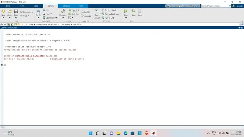
Error occured for missing of the multiplication operator.
2.
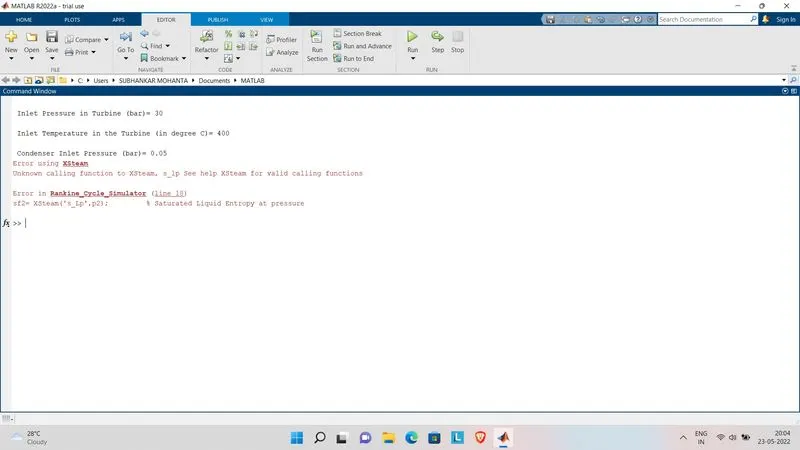
Error mostly occured for calling the wrong function name while extracting value from steam file.
OUTPUT:
The Input parameters:
Inlet pressure at the turbine is 30 bar (P1)
Inlet temperature at the turbine is 400 deg Celcius (T1)
Outlet temperature at the turbine is 0.05 bar (P2)
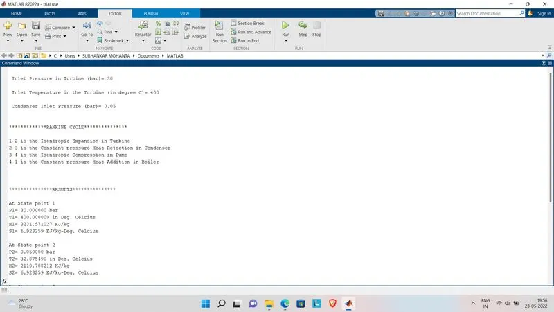
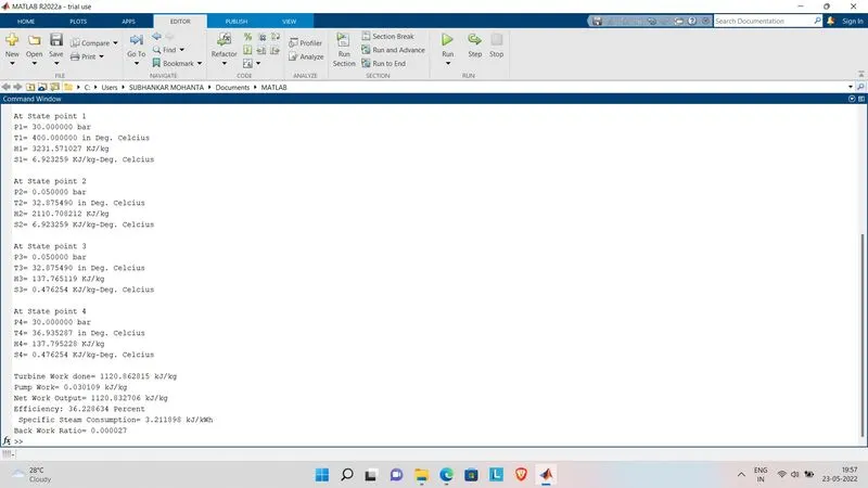
THE GRAPHS:
T-S Diagram:
H-S Diagram:
REFERENCES: