Week 4.1 - Genetic Algorithm

Aim : Try to understand the concept of genetic algorithm.

Objective :

1.Write a code in MATLAB to optimise the stalagmite function and find the global maxima of the function.

2.Clearly expalin the concept of genetic algorithm in your own words and also explain the syntax for ga in MATLAB in your report.

3.Make sure that your code gives the same output, even if it is made to run several times.

Explainations :

In computer science and operations research, a genetic algorithm (GA) is a metaheuristic inspired by the process of natural selection that belongs to the larger class of evolutionary algorithms (EA). Genetic algorithms are commonly used to generate high-quality solutions to optimization and search problems by relying on biologically inspired operators such as mutation, crossover and selection. Some examples of GA applications include optimizing decision trees for better performance, solving sudoku puzzles, hyperparameter optimization, etc.

Genetic Algorithm is a search based optimization technique based on the principle of Genetics and Natural Selection. It is frequently used to find optimal or near-optimal solutions to difficult problems that otherwise would take a lifetime to solve. It is frequently used to solve optimization problems in research and in machine learning.

Nature has always been a great source of inspiration to all mankind Genetic Algorithms (GAs) are search based algorithms based on the concepts of natural selection and genetics.GAs are a subset of a much larger branch of computation known as Evolutionary Computation.

A genetic algorithm is a search heuristic that is inspired by Charles Darwin's theory of natural evaluation. This algorithm reflects the process of natural selection where the fittest individuals are selected for reproduction in order to produce offspring of the next generation.GAs was developed by John Holland and his students and colleagues at the University of Michigan, most notably David E. Goldberg, and has since been tried on various optimization problems with a higher degree of success.

In GAs, we have pooled a population of possible solutions to the given problem. These solutions then undergo recombination and mutation like in natural genetics producing new children and the process is repeated over various generations. Each individual is assigned a fitness value based on its objective function values and the fitter individuals are given a higher chance to mate and yield more fitter individuals. This is in line with the Darwinian Theory of "Survival of the Fittest".In this way, we keep evolving better individuals or solutions over generations till we reach a stopping criterion.

Genetic algorithms are sufficiently randomized in nature but the perform much better than random local search in which we just try various random solutions keeping track of the best so far as they exploit historical information as well.

Advantages of GAs:

GAs have various advantages that have made them immensely popular. These include

1. Does not require any derivative information which may not be available for many real-world problems.
2. Is faster and more efficient as compared to the traditional methods
3. Has very good parallel capabilities
4. Optimizes both continuous and discrete functions and also multi-objective problems
5. Provides a list of good solutions and not just a single solution
6. Always get an answer to the problem which get better over the time
7. Useful when the search space is very large and there are a large number of parameters involved.

Limitations of GAs:

Like any technique GAs also suffer from a few limitations these includes

1. GAs are not suited for all problems especially problems that are simple and for which derivative information is available.
2. The fitness value is calculated repeatedly which might be computationally expensive for some problems.
3. Being stochastic there are no guarantees on the optimality or the quality of the solution.
4. If not implemented properly the GA may not converge to the optimal solution.
5. The genetic algorithm uses three main types of rules at each step to create the next generation from the current population.

Selection rules select the individuals, called parents that contribute to the population at the next generation.

Crossover rules combine two parents to from children for the next generation.

Mutation rules apply random changes to individual parents to the form of children.

The genetic algorithm differs from a classical derivative-based optimization algorithm in two main ways as summarized in the following tables.

Classical Algorithm	Genetic Algorithm
Generates a single point at each iteration. The sequence of points approaches optimal solutions	Generates a population of points at each iteration. The best point in the population approaches an optimal solution
Select the next point in the sequence by a deterministic computation	Select the next population by computation which uses the random number generators.

Descriptions :

in this challenge write code for genetic algorithm

1st write code for x and y variables so create simple array for 0 to 150 for interval 0.6

x = linspace(0,0.6,150)
y = linspace(0,0.6,150)

after that write code for assinging value of inputs by using for loop used i and j variable and also write code for stalagmite functions find f value in here 4 f value f1x,f1y & f2x,f2y f1 for x and y also f2 for x and y

for i = 1:length(x)
for j = 1:length(y)
input(1) = x(i)
input(2) = y(j)
f(i,j)= stalagmite(input)
end
end

used two end close both for loops after that used surfc command and plot the value of the x,y & -f as below

surfc(x,y,-f)
shading interp

this is the code of general genetic algorithm

after that write code for function of stalagmite as below

function [f] = stalagmite(input)
x = input(1);
y = input(2);

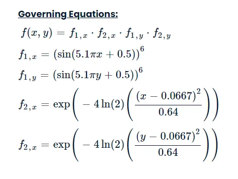
f1x = (sin((5.1*pi*x)+0.5))^6
f1y = (sin((5.1*pi*y)+0.5))^6
f2x = exp(-4*log(2)*(((x-0.0667)^2)/0.64))
f2y = exp(-4*log(2)*(((y-0.0667)^2)/0.64))

f = -(f1x*f1y*f2x*f2y)

here is to find unbounded conditions and bounded conditions in bounded conditions also find value for bounded with population size so write seperate code each other but stalagmite function file used all conditions i.e one file used 3 all conditions

1. case 1 : unbounded

2. case 2 : bounded

3. case 3 : bounded with population size

this all case write seperate code but 1st think is same as mentions above code is used all case is same after that code is small changes

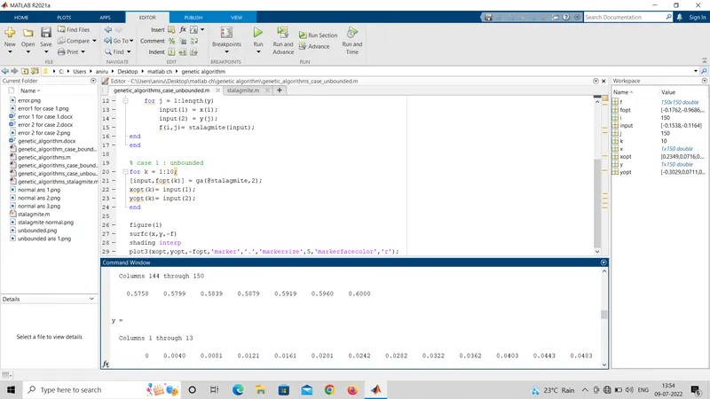
for case 1 : unbounded

for k = 1:10;
[input,fopt(k)] = ga(@stalagmite,2)
xopt(k)= input(1)
yopt(k)= input(2)
end

figure(1)
surfc(x,y,-f)
shading interp
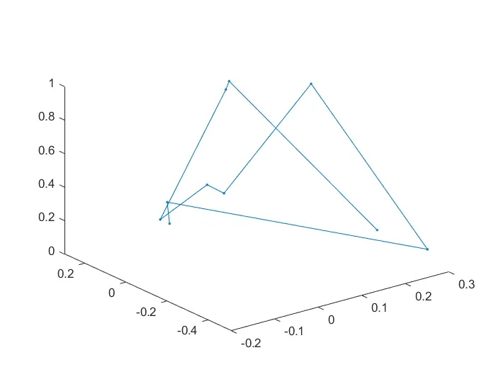
plot3(xopt,yopt,-fopt,'marker','.','markersize',5,'markerfacecolor','r')

this code for case 1 only add polt all 3 point as shown in above and code write using for loop and variables k get xopt, yopt value same thinks follows 2nd case

for case 2 : bounded

for k = 1:10;
[input,fopt(k)] = ga(@stalagmite,2,[],[],[],[],[0;0],[0.4;0.4])
xopt(k)= input(1)
yopt(k)= input(2)
end

surfc(x,y,-f)
shading interp

plot3(xopt,yopt,-fopt,'marker','.','markersize',5)

here only change or adding some thinks in stalagmite functions line i.e add [] this 4 empty bracket as shown because this is a bounded conditions

for case 3 : bounded with population size

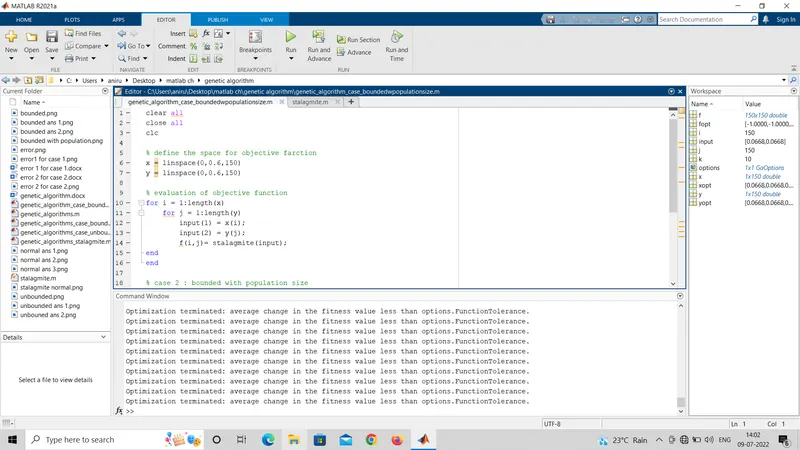
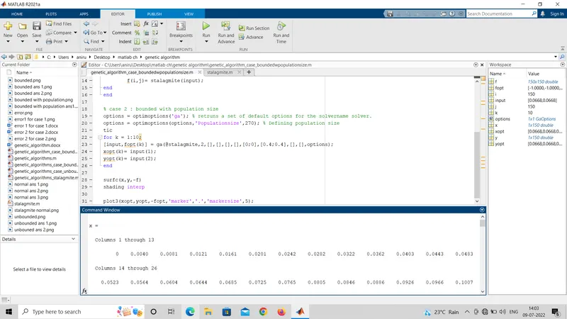
options = optimoptions('ga') .................retruns a set of default options for the solvername solver.
options = optimoptions(options,'Populationsize',270) ............Defining population size
tic
for k = 1:10
[input,fopt(k)] = ga(@stalagmite,2,[],[],[],[],[0;0],[0.4;0.4],[],[],options);
xopt(k)= input(1)
yopt(k)= input(2)
end

surfc(x,y,-f)
shading interp

plot3(xopt,yopt,-fopt,'marker','.','markersize',5)

in this only add the options conditions and size of populations is 270 remaining all thinks is same

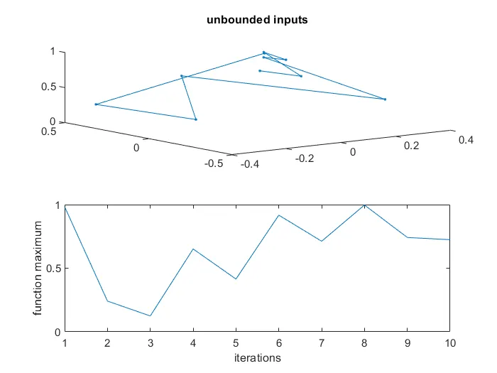
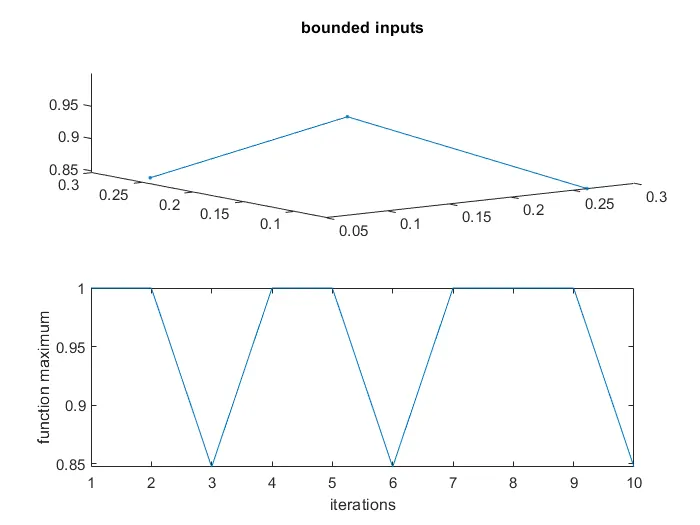
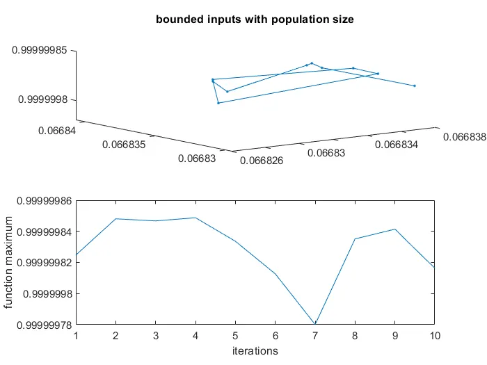
after that write code for Plot graphs for all 3 studies and for F maximum vs no. of iterations. so write a code as below

inthis only add all three studies in one file as below and plot F maximum vs no. of iterations.

in this all initial thinks is same only add all 3 studies code and change in plotting informations so we plotted the F maximum vs no. of iterations easly and this three plot get seprate figure so write in that is figure(1), figure(2), figure(3) on above and also named it that is x label y label and title all graphs .

case 1 : unbounded
for k = 1:10;
[input,fopt(k)] = ga(@stalagmite,2)
xopt(k)= input(1)
yopt(k)= input(2)
end

plotting ga with statistical behaviour

figure(1)
subplot(2,1,1)
surfc(x,y,-f)
shading interp
plot3(xopt,yopt,-fopt,'marker','.','markersize',5,'markerfacecolor','b')
title('unbounded inputs')
subplot(2,1,2)
plot(-fopt)
xlabel('iterations')
ylabel('function maximum')

% case 2 : bounded
for k = 1:10
[input,fopt(k)] = ga(@stalagmite,2,[],[],[],[],[0;0],[0.4;0.4])
xopt(k)= input(1)
yopt(k)= input(2)
end
% plotting ga with statistical behaviour
figure(2)
subplot(2,1,1)
surfc(x,y,-f)
shading interp
plot3(xopt,yopt,-fopt,'marker','.','markersize',5,'markerfacecolor','b')
title('bounded inputs')
subplot(2,1,2)
plot(-fopt)
xlabel('iterations')
ylabel('function maximum')

% case 3 : bounded with population size
options = optimoptions('ga') .........retruns a set of default options for the solvername solver.
options = optimoptions(options,'Populationsize',270) .....Defining population size
tic
for k = 1:10
[input,fopt(k)] = ga(@stalagmite,2,[],[],[],[],[0;0],[0.4;0.4],[],[],options)
xopt(k)= input(1)
yopt(k)= input(2)
end

plotting ga with statistical behaviour
figure(3)
subplot(2,1,1)
surfc(x,y,-f)
shading interp
plot3(xopt,yopt,-fopt,'marker','.','markersize',5,'markerfacecolor','b')
title('bounded inputs with population size')
subplot(2,1,2)
plot(-fopt)
xlabel('iterations')
ylabel('function maximum')

so seen that only changes in plotting thinks

Details code :

function code stalagmite

function [f] = stalagmite(input)
x = input(1);
y = input(2);

f1x = (sin((5.1*pi*x)+0.5))^6;
f1y = (sin((5.1*pi*y)+0.5))^6;
f2x = exp(-4*log(2)*(((x-0.0667)^2)/0.64));
f2y = exp(-4*log(2)*(((y-0.0667)^2)/0.64));

f = -(f1x*f1y*f2x*f2y);

main code

clear all
close all
clc

% define the space for objective farction 
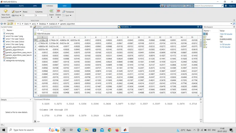
x = linspace(0,0.6,150)
y = linspace(0,0.6,150)

% assinging value of inputs
for i = 1:length(x)
    for j = 1:length(y)
        input(1) = x(i);
        input(2) = y(j);
        f(i,j)= stalagmite(input);
    end
end
surfc(x,y,-f)
shading interp

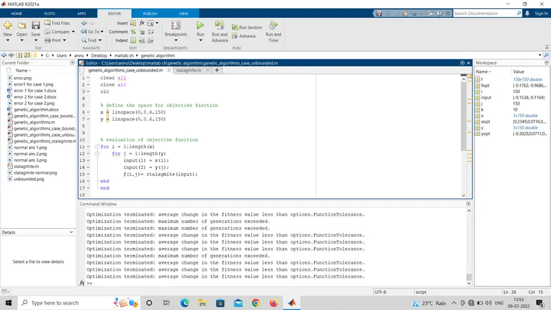
unbounded code

clear all
close all
clc

% define the space for objective farction 
x = linspace(0,0.6,150)
y = linspace(0,0.6,150)


% evaluation of objective function 
for i = 1:length(x)
    for j = 1:length(y)
        input(1) = x(i);
        input(2) = y(j);
        f(i,j)= stalagmite(input);
end
end

% case 1 : unbounded 
for k = 1:10;
[input,fopt(k)] = ga(@stalagmite,2);
xopt(k)= input(1);
yopt(k)= input(2);
end

figure(1)
surfc(x,y,-f)
shading interp
plot3(xopt,yopt,-fopt,'marker','.','markersize',5,'markerfacecolor','r');

bounded code

clear all
close all
clc

% define the space for objective farction 
x = linspace(0,0.6,150)
y = linspace(0,0.6,150)

% evaluation of objective function 
for i = 1:length(x)
    for j = 1:length(y)
        input(1) = x(i);
        input(2) = y(j);
        f(i,j)= stalagmite(input);
end
end

% case 2 : bounded 
for k = 1:10;
[input,fopt(k)] = ga(@stalagmite,2,[],[],[],[],[0;0],[0.4;0.4]);
xopt(k)= input(1);
yopt(k)= input(2);
end

surfc(x,y,-f)
shading interp

plot3(xopt,yopt,-fopt,'marker','.','markersize',5);

bounded with population size code

clear all
close all
clc

% define the space for objective farction 
x = linspace(0,0.6,150)
y = linspace(0,0.6,150)

% evaluation of objective function 
for i = 1:length(x)
    for j = 1:length(y)
        input(1) = x(i);
        input(2) = y(j);
        f(i,j)= stalagmite(input);
end
end

% case 3 : bounded with population size
options = optimoptions('ga'); % retruns a set of default options for the solvername solver. 
options = optimoptions(options,'Populationsize',270); % Defining population size
tic
for k = 1:10;
[input,fopt(k)] = ga(@stalagmite,2,[],[],[],[],[0;0],[0.4;0.4],[],[],options);
xopt(k)= input(1);
yopt(k)= input(2);
end

surfc(x,y,-f)
shading interp

plot3(xopt,yopt,-fopt,'marker','.','markersize',5);

code for Plot graphs for all 3 studies and for F maximum vs no. of iterations

clear all
close all
clc

% define the space for objective farction 
x = linspace(0,0.6,150)
y = linspace(0,0.6,150)

% evaluation of objective function 
for i = 1:length(x)
    for j = 1:length(y)
        input(1) = x(i);
        input(2) = y(j);
        f(i,j)= stalagmite(input);
end
end

% case 1 : unbounded 
for k = 1:10;
[input,fopt(k)] = ga(@stalagmite,2);
xopt(k)= input(1);
yopt(k)= input(2);
end

% plotting ga with statistical behaviour 

figure(1)
subplot(2,1,1)
surfc(x,y,-f)
shading interp
plot3(xopt,yopt,-fopt,'marker','.','markersize',5,'markerfacecolor','b');
title('unbounded inputs')
subplot(2,1,2)
plot(-fopt)
xlabel('iterations')
ylabel('function maximum')

% case 2 : bounded 
for k = 1:10;
[input,fopt(k)] = ga(@stalagmite,2,[],[],[],[],[0;0],[0.4;0.4]);
xopt(k)= input(1);
yopt(k)= input(2);
end
% plotting ga with statistical behaviour
figure(2)
subplot(2,1,1)
surfc(x,y,-f)
shading interp
plot3(xopt,yopt,-fopt,'marker','.','markersize',5,'markerfacecolor','b');
title('bounded inputs')
subplot(2,1,2)
plot(-fopt)
xlabel('iterations')
ylabel('function maximum')

% case 3 : bounded with population size
options = optimoptions('ga'); % retruns a set of default options for the solvername solver. 
options = optimoptions(options,'Populationsize',270); % Defining population size
tic
for k = 1:10;
[input,fopt(k)] = ga(@stalagmite,2,[],[],[],[],[0;0],[0.4;0.4],[],[],options);
xopt(k)= input(1);
yopt(k)= input(2);
end

% plotting ga with statistical behaviour
figure(3)
subplot(2,1,1)
surfc(x,y,-f)
shading interp
plot3(xopt,yopt,-fopt,'marker','.','markersize',5,'markerfacecolor','b');
title('bounded inputs with population size')
subplot(2,1,2)
plot(-fopt)
xlabel('iterations')
ylabel('function maximum')

Results :

1. genetic algoritham without any case only simple code or main code

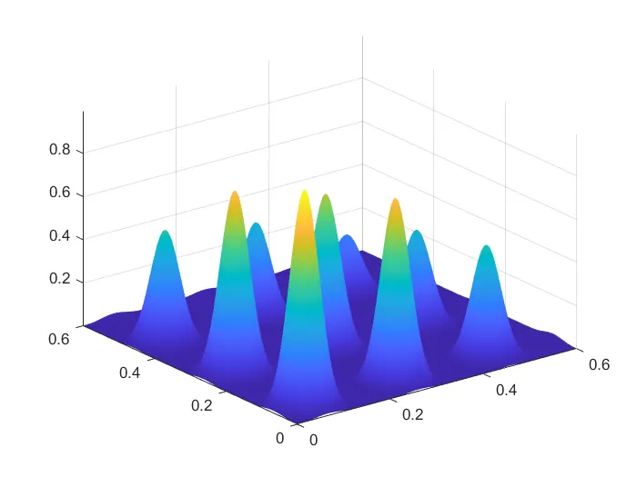
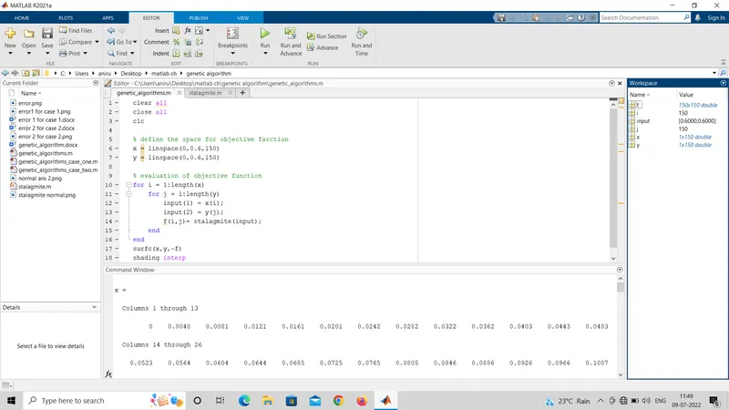
2. unbounded

3. bounded

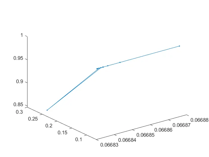
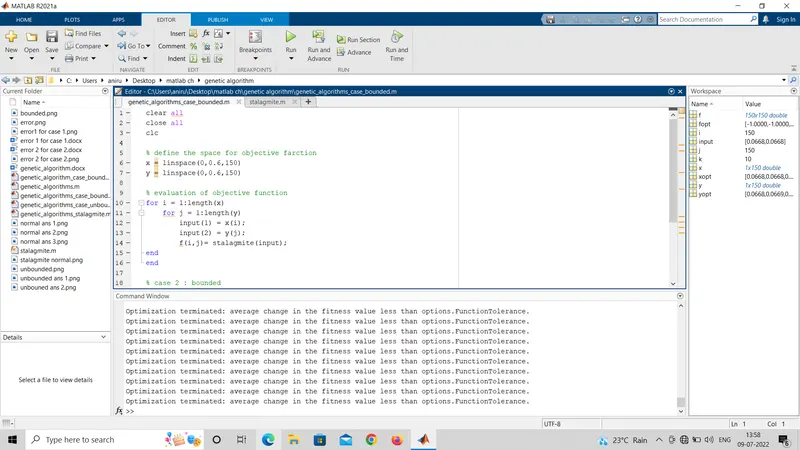
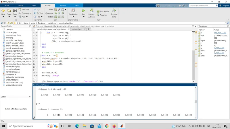
4. bounded with population size

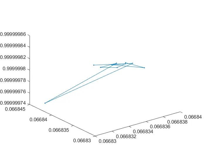
5. plot all three case graphs

Error facing during run program

'stalagmite' is not found in the current folder or on the MATLAB path, but exists in:

C:\Users\aniru\Desktop\matlab ch

Change the MATLAB current folder or add its folder to the MATLAB path.

Error in genetic_algorithms_case_one (line 14)

f(i,j)= stalagmite(input);

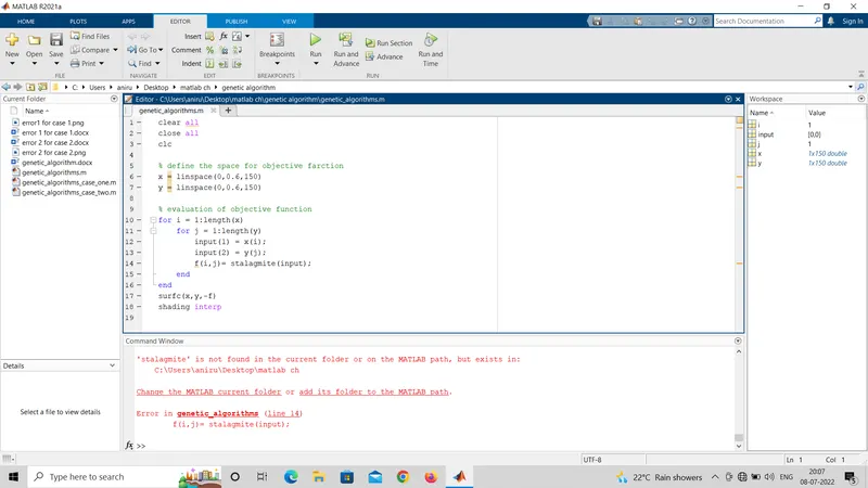
this error so due to stalagmite fuction file saveed other name so matlab not read it so this error show so i saved the file as name as stalagmite and slove error

screen shot of error