Week 4.1 - Genetic Algorithm
Aim: using Genetic algorithm in MATLAB to optimize the stalagmite function and finding the global maxima of the function.
Genetic algorithm:
Genetic algorithm is a stochastic global search method that mimics the metaphor of natural biological evolution. A typical application of GA is to efficiently search a large space of possible solutions to a problems for a optimal solution.
It operates on a population of potential solutions applying the principle of survival of the fittest to produce better and better approximations to a solution. At each generation , a new set of approximations is created by the process of selecting individuals according to their level of fitness in the problem domain and breeding them together using operators borrowed from natural genetics. This process leads to the evolution of populations of individuals that are better suited to their environment.
Steps in Genetic algorithm:
- Initialize population
- Selecting parents by evaluating their fitness
- Crossover parents to reproduce
- Mutating the offspring’s
- Evaluating the offspring’s
- Merge offspring with main population and sort
The main components of the Genetic algorithm are the genotype, phenotype, fitness function, selection algorithm, crossover operator and mutation operator.
Initialization :
The algorithm generally starts with randomly generated solutions. The size of the solutions depends on the nature of the problems. Individual solutions are generally represented by a “genotype”.
Which is processed in software to produce an evaluable “Phenotype”. The genotype is the solutions manipulatable representation, while the phenotype is an evaluable solution to the problem.A genotype chromosome is represented by a software data structure such as a string of bits, characters, integers or real numbers.
Parent selection:
During each successive generation, parents are selected for the existing population to breed new generations. At the start, as there are no offspring’s , parents are selected from the randomly generated solutions. Fitness of the parents are calculated and based on fitness the probability being selected for breeding is calculated. Higher the fitness value higher the probability.
There are 3 main methods to define best fit individuals and select for breeding:
1) Random selection: This is the simplest and most inefficient way of selecting parents. In this method, we shuffle the population by performing permutation and select the first two individuals as parents for breeding. This method is not recommended
2) Tournament selection: This method is based on the probability of selection of each individual. We run several tournaments among a randomly selected group of individuals, select one individual from each group as the winner, and again run the tournament by grouping winners from the first iteration, repeat the process until we converge to two winners parents for breeding. The best member of each group in every iteration has the highest probability of selection.
3)Roulette wheel selection: This is a widely used and most efficient method for selecting parent. It is similar to how roulette wheel works in casinos, drop the ball, spin the wheel, and wait till the wheel stops to see which pot the ball falls in. here we define the probability for each individual of the population or parent based on the fitness value. The probability of each individual is called the fitness of the individual. The arrow is fixed at a place, and the wheel is rotated. When the wheel stops rotating, the parent where the arrow points to is chosen for breeding—the greater the probability larger the area on the wheel, leading to a higher probability of being selected.
The genetic algorithm passes from one generation to the other until the termination criteria of the algorithm is met. The most used criteria for the termination of the algorithm is a fixed maximal number of generations. There is another strategy uses the criteria of the population’s convergence. In general, GA pushes the major part of the population to converge in one single solution. So, when the sum of deviations between individuals becomes smaller than a predefined value, the algorithm can terminate. Also the algorithm may terminate as result of the improvement of the best solution after a certain number of generations. Also, different strategies can be combined together for terminating a genetic algorithm.
Fitness function:
The nature obeys to Darwin’s principle “the survival of the strongest”, i.e., individuals with high fitness value will be reproduces more often compared to those with low fitness value. In GA, the fitness is defined in such a manner that the strongest strings have higher fitness values, and this is used to evaluate each individual of a population. We should highlight here that fitness is the only relationship between GAs and the problem to be solved, and this is the measure to select an individual to be reproduced for the next generation.
Genetic operator:
Genetic operators provide the basic mechanism of searching the GA. Operators are used to create new solutions based on existing solutions to the population. There are two basic types of operators: crossover and mutation.
1) Crossover: Crossover, also called recombination, is an operator that creates new individuals from current population, combining pieces of information coming from different individuals of the population. In fact, it recombines genetic material of two parent individuals to create the offspring of the next generation. When individuals are represented by binary strings , some of the techniques used are single point crossover, multipoint crossover and uniform crossover.
- Single crossover: randomly chooses a point in the strings of both parents, the substrings of the right side of the crossover point are exchanged in order to create 2 new offspring’s.
- Multipoint crossover: several crossover points are randomly selected and exchanged between parents to create new offspring’s.
- Uniform crossover: gene (bit) is selected randomly from one of the corresponding genes of the parent chromosomes. for each bit position in the mask, i.e. its value "1" or "0" indicates that the first parent or second parent contributes to the value of his first successor in that position, and vice versa for the second successor. The crossover between two good solutions may not always yield a better or as good a solution. Since parents are good, the probability of the child being good is high. If offspring is not good (poor solution), it will be removed in the next iteration during “Selection”.
2) Mutation: Mutation is a very easy method to create a new individual. This method can be used after the crossover method. A mutation can be applied in several positions, once a new individual "is born". Mutation does a very simple thing: it replaces one or more genes randomly selected in the individual’s representation. Mutation is done to prevent the GA from falling into local optima, but should not happen very often, because then the GA will actually turn into a random search and thus reduces efficiency .
Evaluating the offspring: After mutation the offering are evaluated to define fitness using cost function.
Genetic algorithm syntax:.
x = ga(fun,nvars,A,b,Aeq,beq,lb,ub,nonlcon,intcon,options)
Input arguments:
fun – Objective function, specified as a function handle or function name. here stalagmite function is used.
nvars - Number of variables, specified as a positive integer.
A - Linear inequality constraints, specified as a real matrix. A is an M-by-nvars matrix, where M is the number of inequalities.Here we use default value []
b - Linear inequality constraints, specified as a real vector. b is an M-element vector related to the A matrix.
Aeq- Linear equality constraints, specified as a real matrix. Aeq is an Me-by-nvars matrix, where Me is the number of equalities.
beq - Linear equality constraints, specified as a real vector. beq is an Me-element vector related to the Aeq matrix.
lb- Lower bounds, specified as a real vector or array of doubles.
ub - Upper bounds, specified as a real vector or array of doubles. ub represents the upper bounds element-wise in lb ≤ x ≤ ub.
nonlcon - Nonlinear constraints, specified as a function handle or function name. nonlcon is a function that accepts a vector or array x and returns two arrays, c(x) and ceq(x).
intcon - Integer variables, specified as a vector of positive integers taking values from 1 to nvars. Each value in intcon represents an x component that is integer-valued.
Options - Optimization options, specified as the output of optimoptions or a structure.
Output arguments :
[x,fval,exitflag,output,population,scores] = ga(___)
x – solution
fval - Objective function value at the solution, returned as a real number. Generally, fval = fun(x).
exitflag - Reason that ga stopped, returned as an integer.
Output- Information about the optimization process.
Population - Final population, returned as a PopulationSize-by-nvars matrix
Scores - final scores, returned as a column vector.
- For non-integer problems, the final scores are the fitness function values of the rows of population.
- For integer problems, the final scores are the penalty fitness values of the population member
Stalamite function:
f(x,y) = −(f1,x⋅f2,x⋅f1,y⋅f2,y)
where,
f1,x= (sin(5.1⋅π⋅x+0.5))6
f1,y= (sin(5.1⋅π⋅y+0.5))6
f2,x=exp(−4⋅log(2)⋅(x−0.0667)2/0.64);
f2,y=exp(−4⋅log(2)⋅(y−0.0667)2/0.64);
Code:
function code
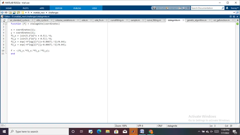
A stalagmite function code is made consisting the above equations where the output solution f(x,y) is calculated.
function [f] = stalagmite(coordinates)

x = coordinates(1);
y = coordinates(2);
f1_x = (sin(5.1*pi*x + 0.5)).^6;
f1_y = (sin(5.1*pi*y + 0.5)).^6;
f2_x = exp(-4*log(2)*((x-0.0667).^2)/0.64);
f2_y = exp(-4*log(2)*((y-0.0667).^2)/0.64);

f = -(f1_x.*f2_x.*f1_y.*f2_y);
end
Main code:
Study -1
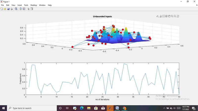
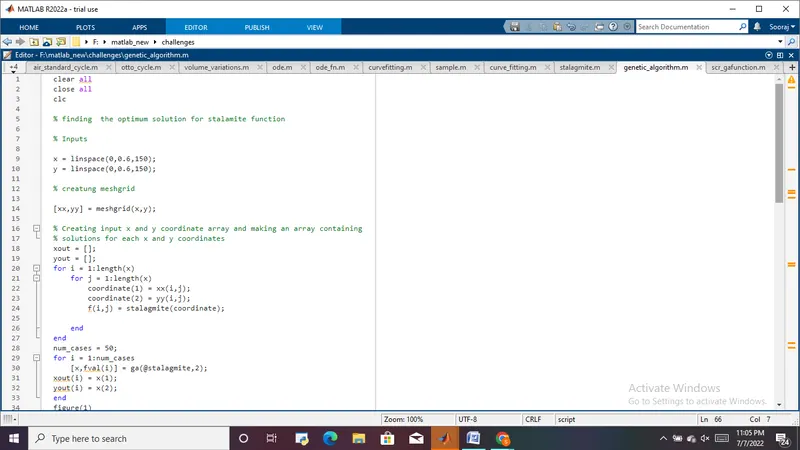
code with no lower bound and upper bound. The genetic algorithm is only given two function and no of variables arguments in the code.
clear all
close all
clc

% finding  the optimum solution for stalamite function

% Inputs

x = linspace(0,0.6,150);
y = linspace(0,0.6,150);

% creatung meshgrid

[xx,yy] = meshgrid(x,y);

% Creating input x and y coordinate array and making an array containing
% solutions for each x and y coordinates
xout = [];
yout = [];
for i = 1:length(x)
    for j = 1:length(x)
        coordinate(1) = xx(i,j);
        coordinate(2) = yy(i,j);
        f(i,j) = stalagmite(coordinate);

    end
end
num_cases = 50;
for i = 1:num_cases
    [x,fval(i)] = ga(@stalagmite,2);
xout(i) = x(1);
yout(i) = x(2);
end
figure(1)
subplot(2,1,1)
surfc(xx, yy, -f)
shading interp
hold on
plot3(xout,yout,-fval,'marker','o','markersize',10,'MarkerFaceColor','r')
title('Unbounded Inputs')
subplot(2,1,2)
plot(-fval)
xlabel('no of iterations')
ylabel('f maximum')
study-2 :
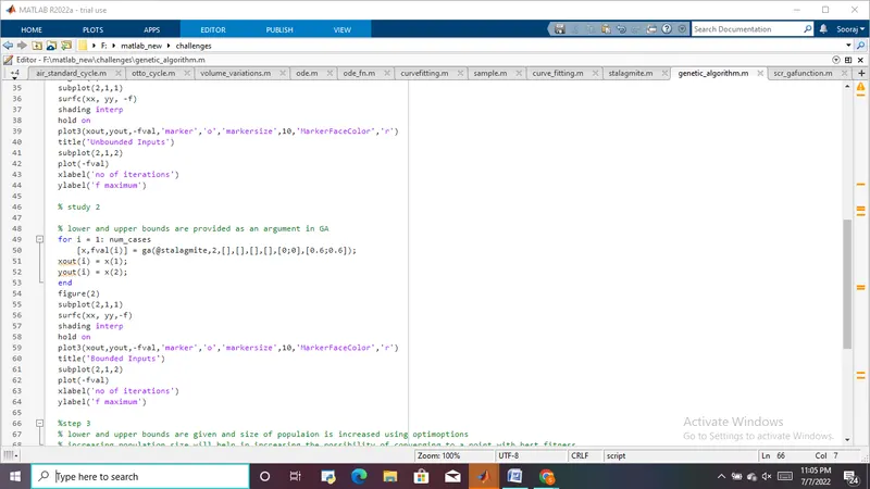
Lower and upper bounds are provided so the solutions are within this range.
% study 2

% lower and upper bounds are provided as an argument in GA
for i = 1: num_cases
    [x,fval(i)] = ga(@stalagmite,2,[],[],[],[],[0;0],[0.6;0.6]);
xout(i) = x(1);
yout(i) = x(2);
end
figure(2)
subplot(2,1,1)
surfc(xx, yy,-f)
shading interp
hold on
plot3(xout,yout,-fval,'marker','o','markersize',10,'MarkerFaceColor','r')
title('Bounded Inputs')
subplot(2,1,2)
plot(-fval)
xlabel('no of iterations')
ylabel('f maximum')
sudy- 3:
Bounded inputs with increased population size
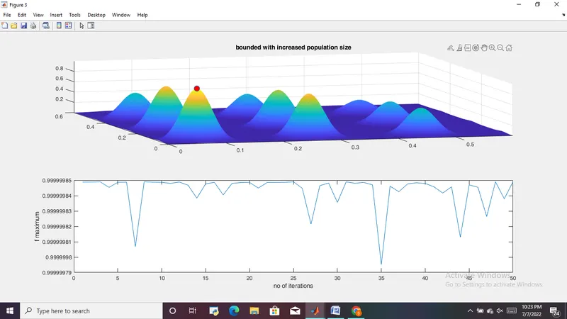
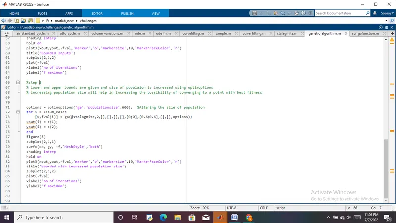
in this case , the upper and lower boundaries are provided , additionally optimoption command is used to alter size of population
%step 3
% lower and upper bounds are given and size of populaion is increased using optimoptions
% increasing population size will help in increasing the possibility of converging to a point with best fitness


options = optimoptions('ga','populationsize',600);  %Altering the size of population
for i = 1:num_cases
    [x,fval(i)] = ga(@stalagmite,2,[],[],[],[],[0;0],[0.6;0.6],[],[],options);
xout(i) = x(1);
yout(i) = x(2);
end
figure(3)
subplot(2,1,1)
surfc(xx, yy, -f,'MeshStyle','both')
shading interp
hold on
plot3(xout,yout,-fval,'marker','o','markersize',10,'MarkerFaceColor','r')
title('bounded with increased population size')
subplot(2,1,2)
plot(-fval)
xlabel('no of iterations')
ylabel('f maximum')
Explanation:
- A function code is made consisting of the above mentioned equations
- Main code is written. It consist of 3 cases .
- first case is unbounded inputs . In unbounded case the genetic algorithm is only given 2 input arguments [ga(fun,nvars)]. Only function code(stalagmite function) and no of variables are provided. then plot of the stalagmite fuction for x and y is made ,then the output values we got using GA is plotted in the same plot.Additional plot of F max vs no of iterations is made .
- 2nd case - bounded input. In this case, in addition to function and no of variables, lower bound and upper bound is also provided . This helps to confine the solution within the range. Then plots are made.
- 3rd case - bounded input with altered population size. in this case , an additional argument ,options is given to genetic algorithm. options is the output of optimoption. optimoption is given an argument 'populationsize' - 500, this means population size is changed to 500. As operation works on a wider population it increase the possibility of finding the better fitness of the function.
Output:
study-1:
Study-2:
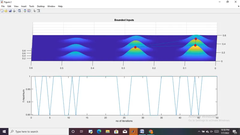
Study 3:
Screenshot of code:
Referance:
- https://www.geeksforgeeks.org/crossover-in-genetic-algorithm/
- https://www.researchgate.net/publication/309616654_The_Genetic_Algorithm_for_finding_the_maxima_of_single-variable_functions
- https://skill-lync.com/student-projects/Genetic-Algorithm-27053
- https://www.mathworks.com/help/gads/ga.html#mw_4a8bfdb9-7c4c-4302-8f47-d260b7a43e26
- https://www.ncbi.nlm.nih.gov/pmc/articles/PMC3813526/
- https://pub.towardsai.net/genetic-algorithm-ga-introduction-with-example-code-e59f9bc58eaf