Challenge

Project 2 - Rankine cycle Simulator

SSooraj V S22 Jul 2022

Aim: Develop a program to calculate the state points of the Rankine cycle from the given inputs, calculate the net work and efficiency of the Rankine cycle and plot T-S and H-S graph of the Rankine cycle.

Theory :

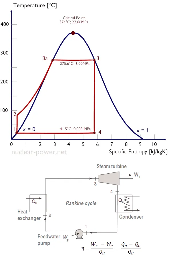
Rankine cycle: the Rankine cycle is an idealized thermodynamic cycle of a constant pressure heat engine that converts part of heat into mechanical work. In this cycle, the heat is supplied externally to a closed loop, which usually uses water (in a liquid and vapor phase) as the working fluid.

From a thermodynamics point of view, the performance of steam turbines can be derived from the theory of the Rankine cycle. Rankine cycle is the fundamental operating cycle of all power plants where an operating fluid is continuously evaporated and condensed .

While many substances could be used as the working fluid in the Rankine cycle (inorganic or even organic), water is usually the fluid of choice due to its favorable properties, such as its non-toxic and unreactive chemistry, abundance, and low cost, as well as its thermodynamic properties.

Rankine cycle consists of 4 processes :

Isentropic expansion in turbine
Isobaric heat rejection by condenser
Isentropic compression in pump
Isobaric heat addition in boiler

1) Isentropic expansion (1-2):

The vapour is expanded in the turbine , thus producing work. In practice , the expansion is limited by the

Temperature of the cooling medium and by the erosion of turbine blades by liquid entrained in he vapour steam as the process moves further in two phase region. In our case we use water as working fluid.

2) Isobaric heat rejection (2-3):

The vapour-liquid mixture leaving the turbine is condensed at low pressure. Usually a surface condenser using cooling water is used.

3) Isentropic compression (3-4):

The pressure of the condensate is raised in the feed pump. Because of low specific volume of liquids, the pump work is relatively small and often neglected in thermodynamic calculation.

4) Isobaric heat addition (4-1):

High pressure liquid enters the boiler from the feed pump and is heated to saturation temperature. Further addition of energy causes evaporation of liquid until it is fully converted to saturated steam .

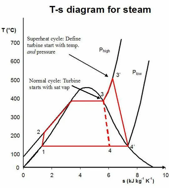
Superheating: superheating is the process in which the vapor of working fluid is heated in boiler to a temperature higher than its boiling point at the absolute pressure where the temperature is measured.

The superheating process is the only way to increase the peak temperature of the Rankine cycle (and to increase efficiency) without increasing the boiler pressure. This requires another type of heat exchanger called a superheater, which produces superheated steam.

Net work: Total work done by the system = work done by turbine - work done by pump

Efficiency : efficiency = work done by turbine/total heat added

heat added(Qin) = h1-h4(heat added in boiler)

Back work ratio: back work ratio is the ratio between the work done by the compressor to the work done by turbine in the thermal power plant.

Code:

clear 
close all
clc

disp(' 1-2 : isentropic expansion in turbine')
disp('2-3 : isobaric heat rejection by condenser')
disp('3-4 : isentropic compression in pump')
disp('4-1 : isobaric heat addition by boiler')
% inputs 
t1 = input('turbine inlet temperature in celsius:');
p1 = input('turbine inlet pressure in bar :');
p2 = input('condensor inlet pressure in bar :');


% Saturated conditions
t1s = XSteam('Tsat_p',p1);
h1_L = XSteam('hL_p',p1);
h1_v = XSteam('hV_p',p1);
h1_lg = h1_v - h1_L;
s1_L = XSteam('sL_p',p1);
s1_v = XSteam('sv_p',p1);
s1_lg = s1_v - s1_L;

h2_L =  XSteam('hL_p',p2);
h2_v = XSteam('hV_p',p2);
h2_lg = h2_v - h2_L;
s2_L = XSteam('sL_p',p2);
s2_v = XSteam('sV_p',p2);
s2_lg = s2_v - s2_L;


% enthalpy at inlet of turbine
h1 = XSteam('h_pT',p1,t1);

% entropy at inlet of turbine
s1 = XSteam('s_pt',p1,t1);

% displaying thermodynamic condition at state 1
disp('RESULTS')
disp('state : 1')
fprintf('pressure is  : %f  bar\n', p1)
fprintf('temperature is  : %f  Deg Celsius\n', t1)
fprintf('Enthalpy is  : %f  Kj/Kg\n', h1)
fprintf('entropy is  : %f  Kj/Kgk\n\n', s1)

% conditions at inlet of condenser
% entropy
s2 = s1;
t2s = XSteam('Tsat_p',p2);
s2s = XSteam('sv_p',p2);
cp2 = XSteam('CpL_p',p2);

% dry fraction
if (s2 < s2_v)
    x2 = (s2 - s2_L)/s2_lg;
else
    x2 = 1;
end
if x2<1
    t2 = t2s;                   % temperature (celsius)
    h2 =  h2_L + (x2*(h2_lg));  % enthalpy (kj/kg)
else
    % saturated steam
    t2 = (t2s+ 273)*exp((s2 - s2_v)/cp2);
    t2 = t2 - 273;
    h2 = h2_v + cp2*(t2 - t2s );
end

% work done by the turbine  = h1 - h2 
Wt = h1 - h2;

% state 2 conditions
disp('state : 2')
fprintf('pressure is  : %f  bar\n', p2)
fprintf('temperature is  : %f  Deg Celsius\n', t2)
fprintf('Enthalpy is  : %f  Kj/Kg\n', h2)
fprintf('entropy is  : %f  Kj/Kgk\n\n', s2)


% state 3
t3 = t2s;
p3 = p2;
v3 = XSteam('vL_p',p3);
s3 = XSteam('sL_T',t3); % entropy (kj/kgk)
h3 = XSteam('hL_T',t3); % enthalpy (kj/kg)

% state 3 conditions
disp('state : 3')
fprintf('pressure is  : %f  bar\n', p3)
fprintf('temperature is  : %f  Deg Celsius\n', t3)
fprintf('Enthalpy is  : %f  Kj/Kg\n', h3)
fprintf('entropy is  : %f  Kj/Kgk\n\n', s3)


% state 4
p4 = p1;
s4 = s3;
cp4 = XSteam('cpl_p',p4);
% workdone by pump
Wp = v3*(p4 - p3)*100;
h4 = Wp + h3;
t4s = XSteam('Tsat_p',p4);  
s4s = XSteam('sL_p',p4);
t4 = t1s/exp((s4s-s4)/cp4);


% state 4 conditions
disp('state : 4')
fprintf('pressure is  : %f  bar\n', p4)
fprintf('temperature is  : %f  Deg Celsius\n', t4)
fprintf('Enthalpy is  : %f  Kj/Kg\n', h4)
fprintf('entropy is  : %f  Kj/Kgk\n\n', s4)

% calculating the efficiency of the rankin cycle
% work by turbine - Wt Kj/kg
% work by pump -Wp kj/Kg
% net work = Wt- Wp
net_W = Wt-Wp;
% heat added to system = h1-h4
Qin = h1 - h4;
% efficiency = net work/heat added
eff = (net_W/Qin)* 100;
% back work ratio = Wp/Wt
BWK = Wp/Wt;
% specific steam consumption
SSC = 3600/Wt;
fprintf('work by turbine : %f Kj/Kg\n',Wt)
fprintf('work by pump : %f Kj/Kg\n',Wp)
fprintf('net work : %f Kj/Kg\n',net_W)
fprintf('efficiency : %f \n',eff)
fprintf('back work ratio : %f \n', BWK)
fprintf('Specific steam consumption : %f Kj/KWh\n',SSC)

% calculating the liquid and vapour line for water
temp = linspace(1,374,500);
for i = 1:length(temp)
    hL(i) = XSteam('hL_T',temp(i)); % enthalpy along the liquid line
    hv(i) = XSteam('hv_T', temp(i)); % enthapy along vapour line
    sL(i) = XSteam('sL_T',temp(i));  % entropy along the liquid line
    sv(i) = XSteam('sv_T',temp(i));  % entropy along vapour line
end
figure(1)
% T-S 
hold on
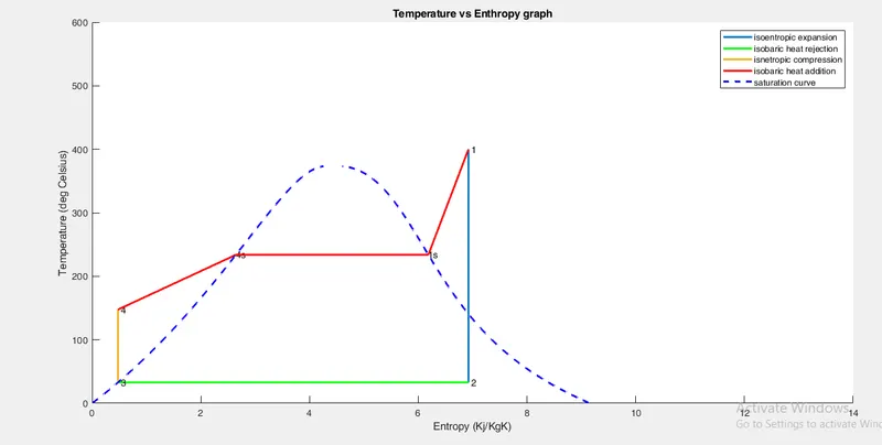
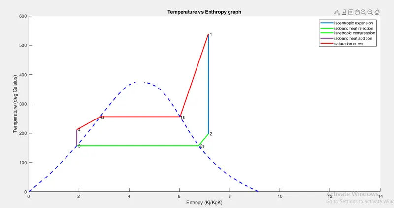
plot([s1,s2],[t1,t2],'LineWidth',2)
text(s1,t1,' 1')
text(s2,t2,' 2')

plot([s2,s3],[t2,t3],'LineWidth',2,'color','g')
text(s3,t3,' 3')
plot([s3,s4],[t3,t4],'LineWidth',2)
text(s4,t4,' 4')
plot([s4,s4s],[t4,t4s],'LineWidth',2,'color','r')
text(s4s,t4s,'4s')
plot([s4s,s1_v],[t4s,t1s],'LineWidth',2,'color','r')
text(s1_v,t1s,'1s')
plot([s1_v,s1],[t1s,t1],'LineWidth',2,'color','r')
plot(sL,temp,'b','LineStyle','--','LineWidth',2)
plot(sv,temp,'b','LineStyle','--','LineWidth',2)
title('Temperature vs Enthropy graph')
xlabel('Entropy (Kj/KgK)')
ylabel('Temperature (deg Celsius)')
legend('isoentropic expansion','isobaric heat rejection','isnetropic compression','isobaric heat addition','','','saturation curve')
axis([0 14 0 600])

% H-S plot 
figure(2)
hold on
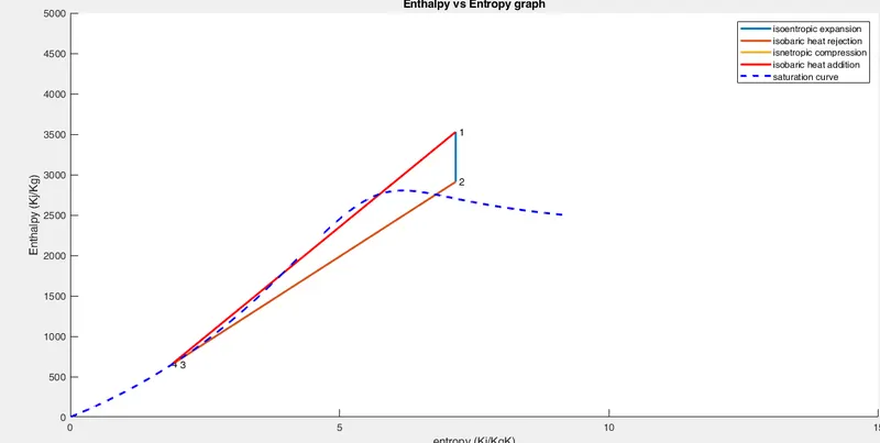
plot([s1,s2],[h1,h2],'LineWidth',2)
text(s1,h1,' 1')
text(s2,h2,' 2')

plot([s2,s3],[h2,h3],'LineWidth',2)
text(s3,h3,'   3')
plot([s3,s4],[h3,h4],'LineWidth',2)
text(s4,h4,'4')
plot([s4,s1],[h4,h1],'LineWidth',2,'color','r')
plot(sL,hL,'b','LineStyle','--','LineWidth',2)
plot(sv,hv,'b','LineStyle','--','LineWidth',2)
title('Enthalpy vs Entropy graph')
xlabel('Entropy (Kj/KgK)')
ylabel('Enthalpy (Kj/Kg)')
legend('isoentropic expansion','isobaric heat rejection','isnetropic compression','isobaric heat addition','saturation curve')
axis([0 15 0 5000])

Explanation:

Xsteam library is given. This library provides accurate steam and water properties from 0 - 1000 bar and from 0 - 2000 deg C according to the standard IAPWS IF-97. For accuracy of the functions in different regions see IF-97
Xsteam function is used to calculate the various thermodynamic properties at a state point
Three input values are given –
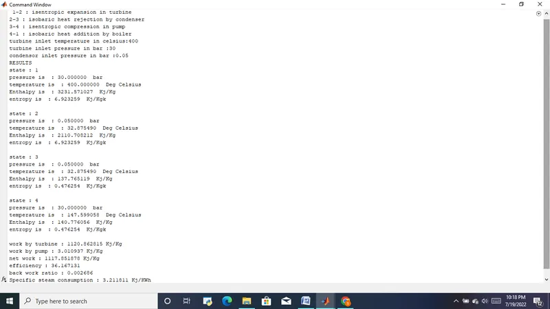
1. temperature at inlet of turbine (t1 - 400 deg Celsius)
2. Pressure at inlet of turbine (p1 - 30bar)
3. Pressure at exit of turbine (p2 - 0.05bar)
Using t1 and p1 values enthalpy and entropy at state one is calculated with help of xsteam function.
Enthalpy(h1) and entropy(s1) of the vapour and liquid line for high pressure(p1) and low pressure (p2) is also calculated
1-2 process is a isentropic process so entropy of state 2 is equal to s1.
To check whether the state 2 is fully saturated( saturated vapour) dry fraction(x2) is calculated
Based on the value of x2 , equation used for calculating enthalpy and temperature varies.
For 3^rd state , temperature is equal to t2(since our case is inside the saturation curve. if not, t3 = t2s) and p3 = p2. With help of xsteam function, the entropy, enthalpy and volume is calculated.
State 4, p4 = p1 and s4 = s3(isentropic compression)
Work done by pump is calculated (w = v*(p 3- p4)). Using work enthalpy h4 is calculate(h4 = w +h3)
Temperature is calculated using given equation.`t4 = t1s/exp((s4s-s4)/(cp4))`
Then net work, efficiency , back work ratio and specific steam consumption is calculated.
Using the state points T-S and H-S plots are made.

Referance:

Plot:

temperature vs entropy diagram

Enthalpy vs Entropy diagram

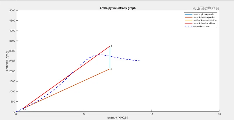
for different inputs(t1 = 538, p1 = 44, p = 5.38)

Output:

Conclusion:

The thermodynamic properties of state points of Rankine cycle are calculated and plot of T-S and H-S diagram is made. superheating results in increasing efficiency of Rankine cycle.

Project 2 - Rankine cycle Simulator

Ship work like this
in your own course.

Talk to a career counsellor

Ship work like thisin your own course.

Talk to a career counsellor

Ship work like this
in your own course.