Week 3 - Solving second order ODEs
AIM: solve the given 2nd order differential equation using
`d^2theta/dt^2 + b/m*d(theta)/dt + g/l*sin(theta)` = 0
& simulate the motion of the pendulum
Theory:
According to Newtons 2nd law of motion
ΣF = Ma : net force ΣF on an object is equal to the object's mass multiplied by acceleration
This lets you set the force of gravitational acceleration (-Mg sin(θ)l) equal to the force of the rotation
ma = `ml^2alpha`
alpha - angular acceleration
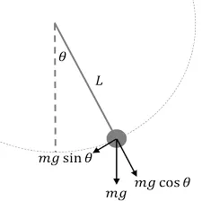
here force of rotation on pendulam = -mgsin(θ)
-mgsin(θ)l = ma
`-mgsin(theta)l = ml^2d^2(theta)/dt^2`
angular acceleration = d2θ/dt2
-mgsin(θ)l = ml*d2θ/dt2
d2θ/dt2 + (g/l)*sin(θ) = 0 ------(1)
When damping factor is involved:
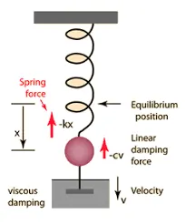
take the case of a mass attached to a spring .one end of the spring is fixed.
Fd is direct proportional to velocity of the mass
fd ∝ v
fd ∝ x'
x' = dx/dt = v
fd = -bx'
here direction of damping is opposite to direction of velocity
net force - fnet = ma
fnet = md2X/ dt2
net force = -kx - bx' (restoring force so given negative sign as it acts opposite to direction of velocity)
k - spring force
-kx - bx' = md2X/ dt2
md2X/ dt2 + kx + b*dx/dt = 0
the equation for simple harmonic motion with damping:
d2X/ dt2 + (k/m)x + (b/m)dx/dt = 0 -----(2)
For simple pendulum with damping coefficient:
combining the (1) and (2)
d2θ/dt2 +(b/m)dθ/dt + (g/l)*sin(θ) = 0
Reducing the order from 2nd order to first order :
θ1 =θ
θ2 = dθ1/dt
therefore equation becomes
dθ2/dt + (b/m)θ2 + (g/l)*sin(θ1) = 0
dθ/dt = -(b/m)θ2 - (g/l)*sin(θ1)
θ1 - angular displacement of pendulum
θ2 - angular velocity of pendulum
d/dt[θ1; θ2]= [θ2 ; -(b/m)θ2 - (g/l)*sin(θ1)]
; - next column
code:
function code:
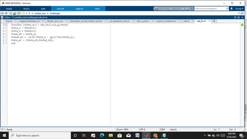
function [theta_ar] = ode_fn(l,m,b,g,theta)
theta_1 = theta(1);
theta_2 = theta(2);
theta_dt = theta_2;
theta2_dt = -(b/m)*theta_2 - (g/l)*sin(theta_1);
theta_ar = [theta_dt;theta2_dt];
endcode for plot and simulation:
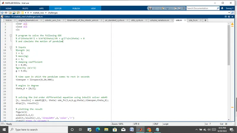
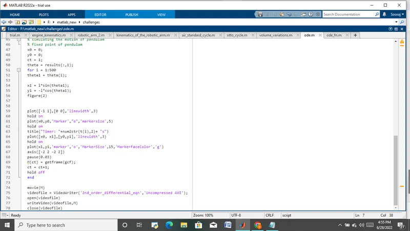
clear all
close all
clc
% program to solve the following ODE
% d^2theta/dt^2 + b/m*d(theta)/dt + g/l*sin(theta) = 0
% and simulate the motion of pendulam
% Inputs
%length (m)
l = 1;
% mass(kg)
m = 1;
% damping coefficient
b = 0.05;
%gravity (m/s^2)
g = 9.81;
% time span in which the pendulam comes to rest in seconds
timespan = linspace(0,20,500);
% angles in degree
theta_0 = [0;3];
% solving the 2nd order differential equation using inbuilt solver ode45
[t, results] = ode45(@(t, theta) ode_fn(l,m,b,g,theta),timespan,theta_0);
disp([t, results])
% plotting the result
figure(1)
subplot(1,2,1)
plot(t,results(:,1),'linewidth',2,'color','r')
xlabel('times in seconds')
ylabel('angular displacement')
title('angular displacement vs time ')
hold on
subplot(1,2,2)
plot(t,results(:,2),'LineWidth',2,'Color','b')
xlabel('times in second')
ylabel('angular velocity')
title('angular velocity vs time')
grid on
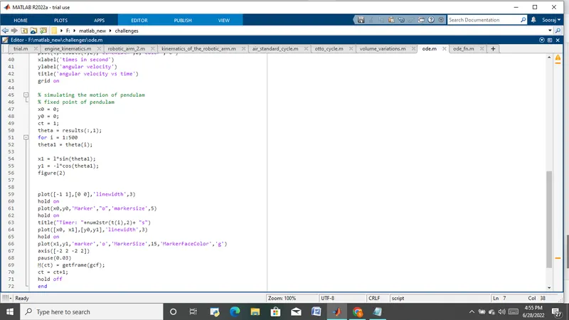
% simulating the motion of pendulam
% fixed point of pendulam
x0 = 0;
y0 = 0;
ct = 1;
theta = results(:,1);
for i = 1:500
theta1 = theta(i);
x1 = l*sin(theta1);
y1 = -l*cos(theta1);
figure(2)
plot([-1 1],[0 0],'linewidth',3)
hold on
plot(x0,y0,'Marker',"o",'markersize',5)
hold on
title("Timer: "+num2str(t(i),2)+ "s")
plot([x0, x1],[y0,y1],'linewidth',3)
hold on
plot(x1,y1,'marker','o','MarkerSize',15,'MarkerFaceColor','g')
axis([-2 2 -2 2])
pause(0.03)
M(ct) = getframe(gcf);
ct = ct+1;
hold o ff
end
movie(M)
videofile = VideoWriter('2nd_order_differential_eqn','Uncompressed AVI');
open(videofile)
writeVideo(videofile,M)
close(videofile)
Explanation:
Inorder to solve a 2nd order differential equation using matlab we must convert the differential equation to first order.
Here , to convert the 2nd order differential equation of pendulum
d2θ/dt2 +(b/m)dθ/dt + (g/l)*sin(θ) = 0
to first order , we wrote a function code. In the function code converted
θ1 =θ
θ2 = dθ1/dt
then the value of theta1 and theta2 are found
d/dt[θ1; θ2]= [θ2 ; -(b/m)θ2 - (g/l)*sin(θ1)]
we got a first order differential equation
then we move on to main program
In the main code we solve the first order differential equation using inbuilt solver ode45.“ode45()” The first argument is the name of the external function that is used to evaluate the right-hand side of the equation. “@(t,x)” in front of the function name is used to denote that “t” and “x” are the names of the time and state variables that are used to evaluate the right-hand side of the equation.The second argument of ode45 is the time vector at which we want to compute the solution, and the third argument is the initial state of the state variable.
[t, results] = ode45(@(t, theta) ode_fn(l,m,b,g,theta),timespan,theta_0)
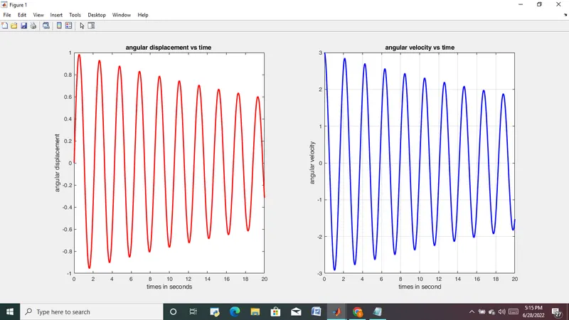
ode45 solves the equation and we get an array of size 500x2, the array consist of 2 columns . 1st column contains angular displacement and 2nd column contains angular velocity.each row contains different angular displacement and angular velocity with respect to time
Then a angular displacement vs time and angular velocity vs time graphs are plotted using the given code
subplot(1,2,1)
plot(t,results(:,1),'linewidth',2,'color','r')
xlabel('times in seconds')
ylabel('angular displacement')
title('angular displacement vs time ')
hold on
subplot(1,2,2)
plot(t,results(:,2),'LineWidth',2,'Color','b')
xlabel('times in second')
ylabel('angular velocity')
title('angular velocity vs time')
grid on
subplot(1,2,1) - one row containing 2 plots and this plot is 1st plot
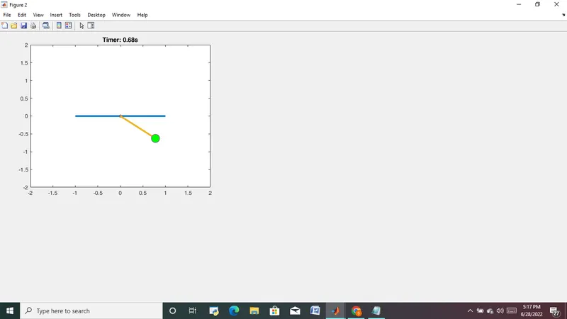
then simulation of motion of pendulum is made. For making the simulation first x0 and y0 is given value 0, this is the fixed end of pendulum.
the coordinates of other end is calculated, a for loop is used to calculated x1 and y1 for each instance of displacement (theta)
theta = results(:,1);
for i = 1:500
theta1 = theta(i);
x1 = l*sin(theta1);
y1 = -l*cos(theta1);
then a line or string is plotted with coordinates x0 y0 at one end and x1 y1 at other end
plot([x0, x1],[y0,y1],'linewidth',3)
to plot a mass at end of string we used marker and markersize code
plot(x1,y1,'marker','o','MarkerSize',15,'MarkerFaceColor','g')
marker - 'o' gives a sphere
markersize - gives size of sphere
then in order to make a animation video
M(ct) = getframe(gcf);
ct = ct+1;
M - an array containing frames of each instance of displacement is made
ct - give position in the array M
movie(M)
videofile = VideoWriter('2nd_order_differential_eqn','Uncompressed AVI');
open(videofile)
writeVideo(videofile,M)
close(videofile)
then a videofile is made by joining different frames in the array M
output:
youtube link:
code:
output: