Week 4.1 - Genetic Algorithm
PROGRAM: GENETIC ALGORITHM
AIM:
To write a code,
- To optimise the stalagmite function and find the global maxima of the function.
- To plot graphs for all 3 studies and for F maximum vs number of iterations.
OBJECTIVE:
- To understand the concept of Genetic Algorithm and syntax for GA in MATLAB.
- To gather information regarding stalagmite function and ways to optimise it.
THEORY:
Genetic Algorithm (GA) is a search-based optimization technique based on the principles of Genetics and Natural Selection. It is frequently used to find optimal or near-optimal solutions to difficult problems which otherwise would take a lifetime to solve. It is frequently used to solve optimization problems, in research, and in machine learning. GAs are a subset of a much larger branch of computation known as Evolutionary Computation.
In GAs, we have a pool or a population of possible solutions to the given problem. These solutions then undergo recombination and mutation (like in natural genetics), producing new children, and the process is repeated over various generations. Each individual (or candidate solution) is assigned a fitness value (based on its objective function value) and the fitter individuals are given a higher chance to mate and yield more “fitter” individuals. This is in line with the Darwinian Theory of “Survival of the Fittest”.
In this way we keep “evolving” better individuals or solutions over generations, till we reach a stopping criterion.
The genetic algorithm is a technique for solving both constrained and unconstrained optimization problems that are based on natural selection, the process that drives biological evolution. The genetic algorithm constantly modifies the population size of individual solutions.
- Phases in Genetic Algorithm:
- Initialization of Population (Coding): The code generates its random population of defined size and from that population the code evaluates the fitness of the members of the population according to which it forms new population based on no. of iterations performed.
- Fitness Function: It is that function which we have to optimize and its optimization is done with the help of number of generations which have been formed by the code accordance with the fitness value of each member generated, these fitness values are used for the reproduction of the children.
- Selection: The idea of the selection phase is to select the fittest individuals and let them pass their genes to the next generation. The main goal of this phase is to find the region where the chances of getting the best solution are more.
Inspiration for this is from the survival of the fittest, It should be a balance between exploration and exploitation of search space, GA tries to move the genotype to higher fitness in the search space ,Too strong fitness selection bias can lead to sub-optimal solutions, Too little fitness bias selection results in unfocused search.
- Reproduction:
Generation of offspring happen in 2 way: Crossover and Mutation.
1). Crossover: Crossover is the most significant stage in the genetic algorithm. During crossover, a random point is selected while mating a pair of parents to generate offspring. There are 3 major types of crossover.
Single Point Crossover: A point on both parents’ chromosomes is picked randomly, and designated a ‘crossover point’.
Two-Point Crossover: Two crossover points are picked randomly from the parent chromosomes.
Unifofm Crossover: In a uniform crossover, typically, each bit is chosen from either parent with equal probability.
2). Mutation: In a few new offspring formed, some of their genes can be subjected to a mutation with a low random probability. This indicates that some of the bits in the bit chromosome can be flipped. Mutation happens to take care of diversity among the population and stop premature convergence.
Syntax:
x = ga(fun,nvars)
x = ga(fun,nvars,A,b)
x = ga(fun,nvars,A,b,Aeq,beq)
x = ga(fun,nvars,A,b,Aeq,beq,lb,ub)
x = ga(fun,nvars,A,b,Aeq,beq,lb,ub,nonlcon)
x = ga(fun,nvars,A,b,Aeq,beq,lb,ub,nonlcon,options)
x = ga(fun,nvars,A,b,Aeq,beq,lb,ub,nonlcon,intcon)
x = ga(fun,nvars,A,b,Aeq,beq,lb,ub,nonlcon,intcon,options)
x = ga(problem)
[x,fval] = ga(___)
[x,fval,exitflag,output] = ga(___)
[x,fval,exitflag,output,population,scores] = ga(___)
x= ga(fun,nvars)x, to the objective function,fun.nvarsis the dimension (number of design variables) offun.x= ga(fun,nvars,A,b,Aeq,beq)xtofun, subject to the linear equalitiesAeq*x=beqandA*x≤b. (SetA=[]andb=[]if no linear inequalities exist.)gaevaluates the matrix productAeq*xas ifxis transposed (Aeq*x').x= ga(fun,nvars,A,b,Aeq,beq,lb,ub)x, so that a solution is found in the rangelb≤x≤ub. (SetAeq=[]andbeq=[]if no linear equalities exist.)
x= ga(fun,nvars,A,b,Aeq,beq,lb,ub,nonlcon)nonlcon. The functionnonlconacceptsxand returns vectorsCandCeq, representing the nonlinear inequalities and equalities respectively.gaminimizes thefunsuch thatC(x)≤0andCeq(x) = 0. (Setlb=[]andub=[]if no bounds exist.)x= ga(fun,nvars,A,b,Aeq,beq,lb,ub,nonlcon,options)options. (Setnonlcon=[]if no nonlinear constraints exist.) Createoptionsusingoptimoptions.
x= ga(fun,nvars,A,b,Aeq,beq,lb,ub,nonlcon,intcon)x= ga(fun,nvars,A,b,Aeq,beq,lb,ub,nonlcon,intcon,options)intcontake integer values.
[also returns a matrixx,fval,exitflag,output,population,scores] = ga(___)population, whose rows are the final population, and a vectorscores, the scores of the final population.
Outline summary of working of GA:
- The algorithm begins by creating a random initial population.
- The algorithm then creates a sequence of new populations. At each step, the algorithm uses the individuals in the current generation to create the next population. To create the new population, the algorithm performs the following steps:
- Scores each member of the current population by computing its fitness value. These values are called the raw fitness scores.
- Scales the raw fitness scores to convert them into a more usable range of values. These scaled values are called expectation values.
- Selects members, called parents, based on their expectation.
- Some of the individuals in the current population that have lower fitness are chosen as elite. These elite individuals are passed to the next population.
- Produces children from the parents. Children are produces either by making random changes to a single parent - mutation - or by combining the vector entries of a pair of parents - crossover.
- Replaces the current population with the children to form next generation.
- The algorithm stops when one of the stopping criteria is met.
GOVERNING EQUATIONS:
Stalagmite Function:
`f(x,y)=f_(1,x).f_(2, x).f_(1, y).f_(2, y)`
where,
`f_(1,x)=[sin(5.1pix+0.5)]^6`
`f_(1,y)=[sin(5.1piy+0.5)]^6`
`f_(2,x)= exp[-4ln(2)(x-0.0667)^2/0.64]`
`f_(2,y)= exp[-4ln(2)(y-0.0667)^2/0.64]`
- A stalagmite is an upward growing mound of mineral deposites that have precipitated from water dripping onto the floor of a cave. Most stalagmites have rounded or flattened tips.
- A stalagmite function generally refers to the function with which we are generating values over a stalagmite kind of surface for finding out the local and global maxima and minima of that particular given function.
- For this in Matlab we are using a method called 'Optimization'. It is a programming which does a selection of the best element with regard to some criterion from some set of population.
- Optimization is done by systematically choosing input values from within an allowed set and computing the results of the function.
-
In matlab to perform optimization we use 'Genetic Algorithm 'method which is a inbuild function in matlab to find the global maxima of that given stalagmite function.
STALAGMITE FUNCTION CODE:
function  [F] = stalagmite(input_vector)
x=input_vector(1);
y=input_vector(2);
f1_x=(sin(5.1*pi*x+0.5)).^6;
f2_x=exp((-4*log(2)*((x-0.0667).^2))/0.64);
f1_y=(sin(5.1*pi*y+0.5)).^6;
f2_y=exp((-4*log(2))*((y-0.0667).^2)/0.64);
F =-(f1_x.*f2_x.*f1_y.*f2_y);
end- Explanation:
Initially, the stalagmite function was mentioned with appropriate argument vectors and saved in the same folder of main code.
While using the function at the end as we are using the -ve sign so that the plot will be reversed as we have to find the maxima of the given function using ga.
MAIN CODE:
close all
clear all
clc

% Inputs
X=linspace(0,0.6,150);
Y=linspace(0,0.6,150);

% Iteration count
num_cases = 60;

% Creating a 2D array
[xx yy] = meshgrid(X,Y);
% Creating input x and y coordinate array and making an array containing
% solutions for each x and y coordinates
xout =[];
yout =[];
for i=1:length(X)
    for j=1:length(Y)
        input_vector(1)=xx(i,j);
        input_vector(2)=yy(i,j);
        f(i,j)=stalagmite(input_vector);
    end
end

% Study-1 : Unbounded inputs

for m=1:num_cases
    [x,fval(m)]=ga(@stalagmite,2);
    xout(m)=x(1);
    yout(m)=x(2);
end

figure(1)
subplot(2,1,1)
surfc(xx,yy,-f)
shading interp
hold on
plot3(xout,yout,-fval,'Marker','o',MarkerSize=5,MarkerFaceColor='g')
subplot(2,1,2)
plot(-fval)
xlabel('Number of Iteration')
ylabel('Function maximum')
title('Unbounded Inputs','FontSize',12)


% Study-2: Bounded inputs

for k=1:num_cases
    [x,fval(k)]=ga(@stalagmite,2,[],[],[],[],[0;0],[0.6;0.6]);
    xout(k)=x(1);
    yout(k)=x(2);
end

figure(2)
subplot(2,1,1)
surfc(xx,yy,-f)
shading interp
hold on
plot3(xout,yout,-fval,'Marker','o',MarkerSize=5,MarkerFaceColor='g')
subplot(2,1,2)
plot(-fval)
xlabel('Number of Iteration')
ylabel('Function maximum')
title('Bounded Inputs','FontSize',12)

% Study-3: Bounded with increased initial population
% lower and upper bounds are given and size of populaion is increased using optimoptions
% Increasing population size will help in increasing the possibility of converging to a point with best fitness

options=optimoptions('ga','PopulationSize',500)
for l=1:num_cases
    [x,fval(l)]=ga(@stalagmite,2,[],[],[],[],[0;0],[0.6;0.6],[],[],options);
    xout(l)=x(1);
    yout(l)=x(2);
end

figure(3)
subplot(2,1,1)
surfc(xx,yy,-f,'MeshStyle','both')
shading interp
hold on
plot3(xout,yout,-fval,'Marker','o',MarkerSize=5,MarkerFaceColor='g')
subplot(2,1,2)
plot(-fval)
xlabel('Number of Iteration')
ylabel('Function maximum')
title('Increased initial population','FontSize',12)
- Explanation:
- The program has been subdivided into three studies based on the limitations of the previous study.
- First study deals with unbounded inputs, thereby expanding the boundary wherein the results can be obtained.
- Second study brings in the aspect of bounded inputs providing a better solution for the drawback faced.
- Third study lays a appreciable platform to determine the exact solution.
- Plots of all the three studies have been displayed, thus giving a clear insight of the results.
- First we initialise the values of x and y taking 150 values between the interval 0 and 0.6. We consider no of iterations as num_cases=60.
% InputsX=linspace(0,0.6,150);Y=linspace(0,0.6,150);% Iteration countnum_cases = 60; - Since we need to plot a 3D surface plot, we take the 2d array of x and y using meshgrid command and store them in input_vector array ,so that it can be used as an argument to call the function stalagmite.
% Creating a 2D array[xx yy] = meshgrid(X,Y);% Creating input x and y coordinate array and making an array containing% solutions for each x and y coordinatesxout =[];yout =[];for i=1:length(X)for j=1:length(Y)input_vector(1)=xx(i,j);input_vector(2)=yy(i,j);f(i,j)=stalagmite(input_vector);endend
We also call the stalagmite function to take the output as f. Here we use -f, because the ga gives us the maximum. - FIRST STUDY: In the first study we take unbounded inputs. Here the number of iteration is number of cases. We uses GA function to calculate the maximum of the function.
we store the outputs into 'x' which contain maximas and 'fval' which contain the value at which the maxima is obtained.
Here the ga is initiated with random population.
% Study-1 : Unbounded inputsfor m=1:num_cases[x,fval(m)]=ga(@stalagmite,2);xout(m)=x(1);yout(m)=x(2);endfigure(1)subplot(2,1,1)surfc(xx,yy,-f)shading interphold onplot3(xout,yout,-fval,'Marker','o',MarkerSize=5,MarkerFaceColor='g')subplot(2,1,2)plot(-fval)xlabel('Number of Iteration')ylabel('Function maximum')title('Unbounded Inputs','FontSize',12)
store the results into xout, yout. Then plot the surface of x,y,-f to get the 3D plot. surfc command is used.
We use the plot3 command to make a plot of xout, yout and -fval to plot the optimum maximas.
Also let us plot the fval function so that we can visualise the optimum values at each iteration.
- SECOND STUDY: Here we consider the bounded inputs, i.e. specify the lower and upper bounds of x and y in this case,the ga is initiated with random population only.
As we store the results earlier we use different syntax for ga, to specify the upper and lower boundaries. The plot is also made as we plot the graph for the first case.
% Study-2: Bounded inputs
for k=1:num_cases[x,fval(k)]=ga(@stalagmite,2,[],[],[],[],[0;0],[0.6;0.6]);xout(k)=x(1);yout(k)=x(2);endfigure(2)subplot(2,1,1)surfc(xx,yy,-f)shading interphold onplot3(xout,yout,-fval,'Marker','o',MarkerSize=5,MarkerFaceColor='g')subplot(2,1,2)plot(-fval)xlabel('Number of Iteration')ylabel('Function maximum')title('Bounded Inputs','FontSize',12) - THIRD STUDY: Bounded inputs and increased population size.
Here in this case to set a initial population we need to use command called optimoptions and get our value of 'populationsize' to 500.
Then store the xout, yout and fval. By using surfc and plot commands the graph is made.
% Study-3: Bounded with increased initial population% lower and upper bounds are given and size of populaion is increased using optimoptions% Increasing population size will help in increasing the possibility of converging to a point with best fitnessoptions=optimoptions('ga','PopulationSize',500)for l=1:num_cases[x,fval(l)]=ga(@stalagmite,2,[],[],[],[],[0;0],[0.6;0.6],[],[],options);xout(l)=x(1);yout(l)=x(2);endfigure(3)subplot(2,1,1)surfc(xx,yy,-f,'MeshStyle','both')shading interphold onplot3(xout,yout,-fval,'Marker','o',MarkerSize=5,MarkerFaceColor='g')subplot(2,1,2)plot(-fval)xlabel('Number of Iteration')ylabel('Function maximum')title('Increased initial population','FontSize',12)
- Code:
a) Stalagmite Function code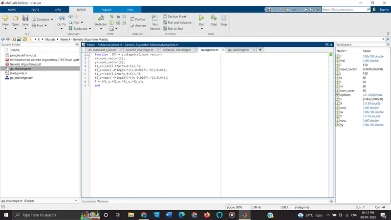
b) Main code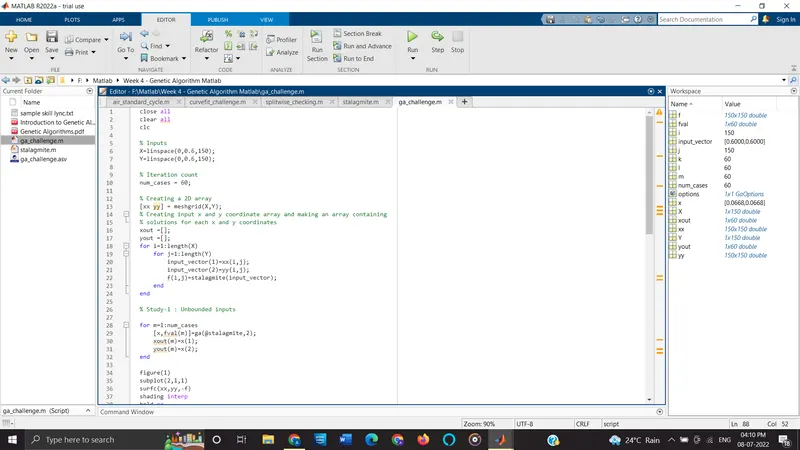
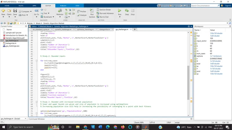
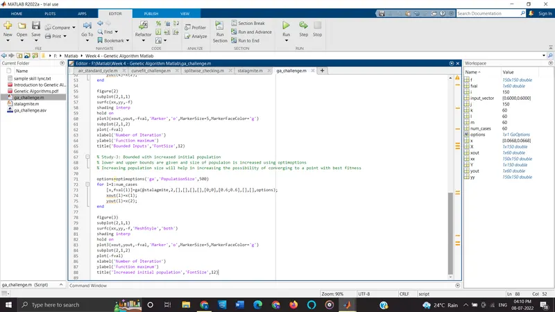
- Code with graph:
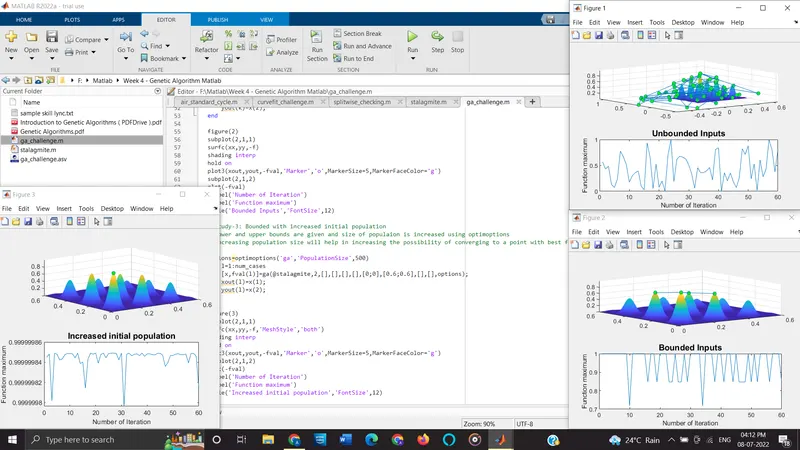
- Diagram:
a) Study-1: Unbounded inputs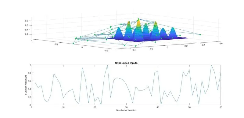
The results obtained for the unbounded inputs vary over a large sized interval. But it can be observed that the value of function maximum lies between the interval 0 and 1. Here, in the study-1, the solutions are not bounded so the GA will calculate all the possible maxima in 'x' and 'y' coordinates.
b)Study-2: Bounded inputs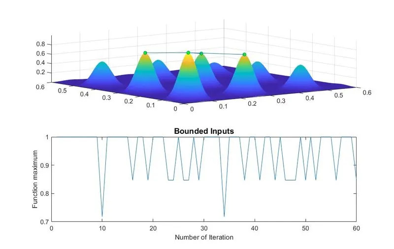
As the solution is dispersed in space we are limiting it to the global maxima simply we are converging the area for GA function for optimum values, on iterating the for loop for 60 times means, we are evolving our solution to get better results for every generation to generation.
c)Study-3: Bounded inputs and increased population size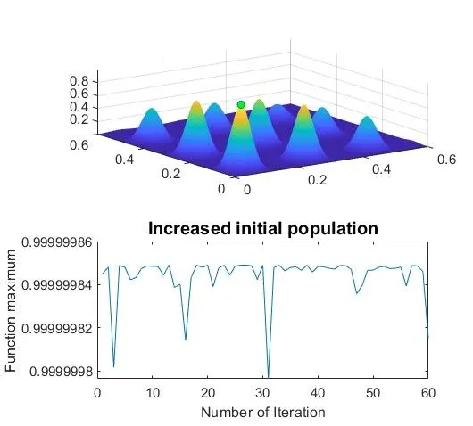
The time taken for execution of function is more. By increasing the size of initial population of ga, we can increase the accuracy of the algorithm. Assumed value of population size is taken as 500.
RESULT:
- The code to optimise the stalagmite function and find the global maxima of the function is made.
- The graphs for all 3 studies and for F maximum vs number of iterations were plotted.
- The concept of Genetic Algorithm and syntax for GA in MATLAB were studied.
CONCLUSION:
- By increasing the population size of GA, the stalagmite function can be optimized.
- For bounded inputs, we gave lower and upper boundaries. So the global maxima simply we are converging the area for GA function for optimum values.
- In the study-3, increased initial population size is given with bounded inputs. So we can increase the accuracy of the algorithm.
REFERENCES:
- https://in.mathworks.com/help/gads/genetic-algorithm.html
- Introduction to Genetic Algorithms, S.N.Sivanandam and S.N.Deepa
- https://towardsdatascience.com/introduction-to-genetic-algorithms-including-example-code-e396e98d8bf3
- https://in.mathworks.com/help/gads/ga.html
- https://www.tutorialspoint.com/genetic_algorithms/genetic_algorithms_parent_selection.htm