Week 3 - Solving second order ODEs
PROGRAM: SOLVING SECOND ORDER ODEs
AIM:
To write a program which,
- Solves the ODE which represents the equation of motion of a simple pendulum with damping.
- Simulate the pendulum motion and save it as video.
THEORY AND GOVERNING EQUATION:
A simple pendulum consists of a ball (point-mass) m, hanging from a (massless) string of length l and fixed at a pivot point P. When displaced to an initial angle and released, the pendulum will swing back and forth with periodic motion. By applying Newton's secont law for rotational systems,we can get the equation of motion for the pendulum.
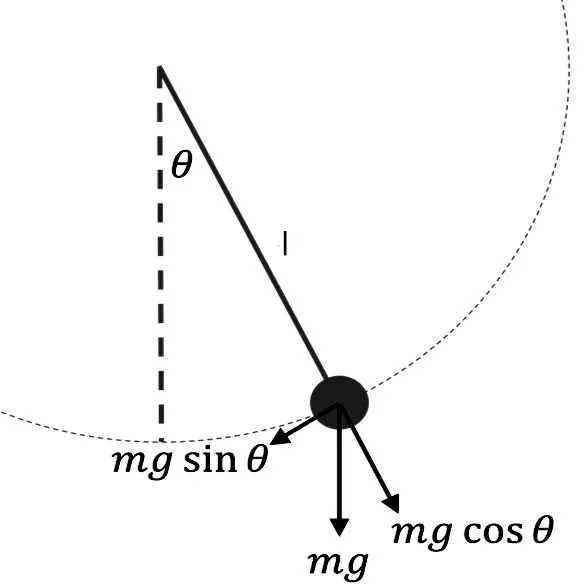
The primary forces acting on the bob are the gravitational force that makes it move in the first place and the force exerted by the string to keep it moving along a circular path. In addition, there may be a damping force from friction at the pivot or air resistance or both. We will construct a model to describe how the angle `theta` of the pendulum varies as a function of time t.
Let s(t) be the distance along the arc from the lowest point to the position of the bob at time t, with displacement to the right considered positive. Let `theta`(t) be the corresponding angle with respect to the vertical. The figure shows tangential and radial components of gravitational force on the pendulum bob. The radial component is exactly balanced by the force exerted by the string, so the only relevant force producing the motion is the tangential component of the gravitational force. For the moment, we ignore the damping force, if any.
The gravitational force is directed downward and has magnitude mg (mass x acceleration), where g is the gravitational acceleration constant, 9.81 m/`s^2` near sea level. Thus, the force acting in the tangential direction is -mg sin(`theta`). (The negative sign is because this force is in the negative direction when `theta` is positive and vice versa.) Since this force is mass x acceleration, it follows that
`(d^2s)/dt^ 2 = -g*sintheta`
Now s and `theta` are related as arc length and central angle in a circle of radius l: s = l* `theta`. Thus, the second derivative of s is l times the second derivative of `theta`. That brings us to our undamped model differential equation with a single dependent variable, the angular displacement `theta`:
`(d^2theta)/dt^2 = -(g/l)*sintheta`
Next, we add damping to the model. We make the simplest possible assumption about the damping force, that it is proportional to velocity. We will represent the damping as proportional to angular velocity. The negative sign is because the damping force has to be opposite the direction of motion. When we include this term in the model, our equation becomes,
`(d^2theta)/dt^2 = -b/m*(d theta)/dt- g/l*sintheta`
`implies (d^2theta)/dt^2 +b/m*(d theta)/dt+ g/l*sintheta=0`
This is a second order ODE. So for solving this in Matlab we breakdown this into two first order ODE. Then it solves by using inbuilt solver ode45() in Matlab.
i.e. taking, `theta = theta_1`
`(d theta)/dt= (d theta_1)/dt=theta_2`
`(d^2 theta)/dt^2 = (d^2 theta_1)/dt^2=(d theta_2)/dt`
FUNCTION CODE:
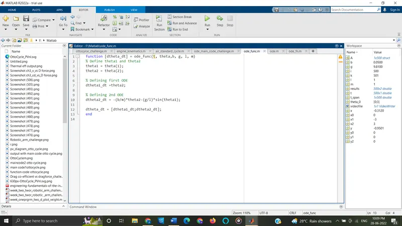
function [dtheta_dt] = ode_func(t, theta,b, g, l, m)
% Define theta1 and theta2
theta1 = theta(1);
theta2 = theta(2);

% Defining first ODE
dtheta1_dt =theta2;

% Defining 2nd ODE
dtheta2_dt = -(b/m)*theta2-(g/l)*sin(theta1);

dtheta_dt = [dtheta1_dt;dtheta2_dt];
end
MAIN CODE:
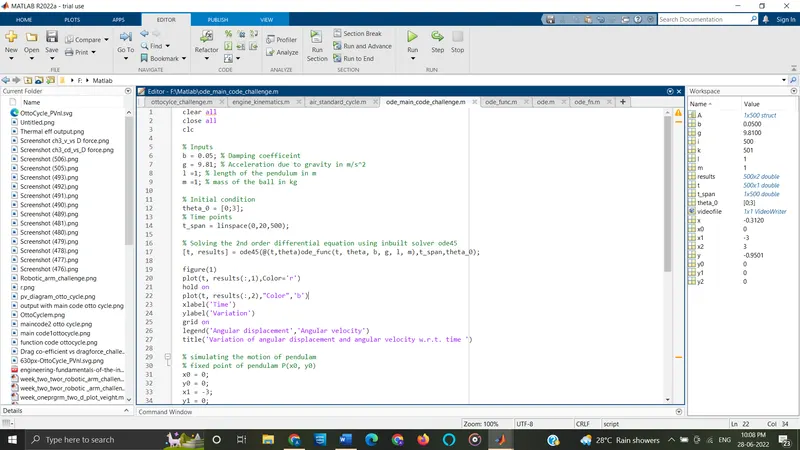
clear all
close all
clc

% Inputs
b = 0.05; % Damping coefficeint
g = 9.81; % Acceleration due to gravity in m/s^2
l =1; % length of the pendulum in m
m =1; % mass of the ball in kg

% Initial condition
theta_0 = [0;3];
% Time points
t_span = linspace(0,20,500);

% solving the 2nd order differential equation using inbuilt solver ode45
[t, results] = ode45(@(t,theta)ode_func(t, theta, b, g, l, m),t_span,theta_0);

figure(1)
plot(t, results(:,1),Color='r')
hold on
plot(t, results(:,2),"Color",'b')
xlabel('Time')
ylabel('Variation')
grid on
legend('Angular displacement','Angular velocity')
title('Variation of angular displacement and angular velocity w.r.t. time ')

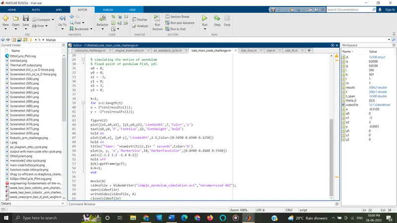
% simulating the motion of pendulam
% fixed point of pendulam P(x0, y0)
x0 = 0;
y0 = 0;
x1 = -3;
y1 = 0;
x2 = 3;
y2 = 0;

k=1;
for i=1:length(t)
x = l*sin(results(i));
y = -l*cos(results(i));

figure(2)
plot([x1,x0,x2], [y1,y0,y2],'LineWidth',7,'Color','y')
text(x0,y0,'P','FontSize',12,'FontWeight','bold')
hold on
plot([x0,x], [y0 y],'LineWidth',2.5,Color=[0.9290 0.6940 0.1250])
hold on
title("Timer: "+num2str(t(i),2)+ " seconds",Color='b')
plot(x, y, 'o','MarkerSize',18,'MarkerFaceColor',[0.4940 0.1840 0.5560])
axis([-3.2 3.2 -1.4 0.2])
hold off
A(k)=getframe(gcf);
k=k+1;
end

movie(A)
videofile = VideoWriter("simple_pendulum_simulation.avi","Uncompressed AVI");
open(videofile)
writeVideo(videofile, A)
close(videofile)
EXPLANATION:
- Function code:
Here the function code is used to breakdown the second order ODE into two first order ODE.
Initially the function ode_func recieves the values for t, `theta`,b , g, l and m. Then it will define the `theta_1 and theta_2`as explained in the theory section.
- Main code:
The main code initially inputs given values of damping coefficient (b) = 0.05, acceleration due to gravity (g) = 9.81 m/`s^2`, length of pendulam (l) =1 m and mass ball (m) =1 kg.
- Function code:
- Main code:
- Code with diagram:
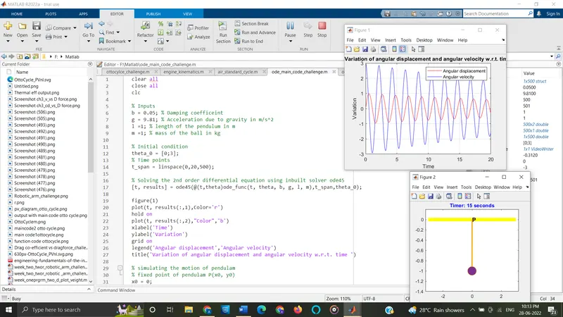
- Output Diagram:
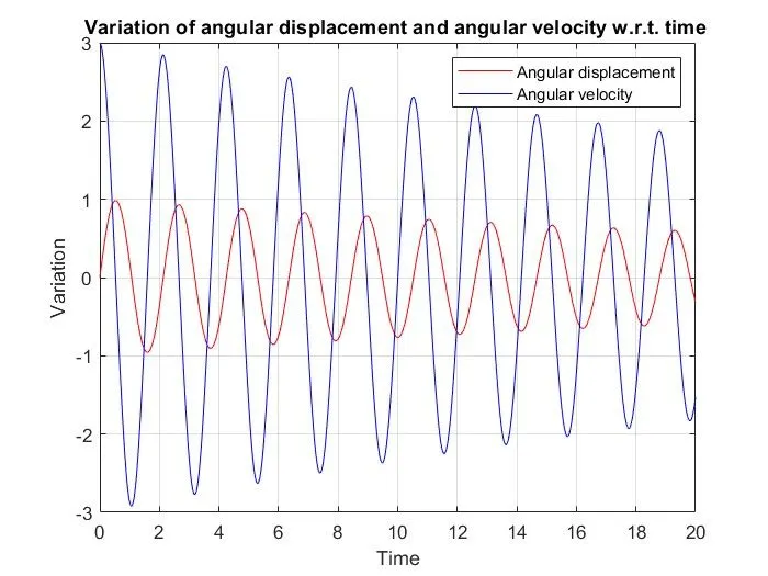
The graph shows the variation of angular velocity and angular displacement within the time interval 0 to 20 seconds. We can clearly understand that initially the pendulum started at 0 angular displacement and 3 rad/s angular velocity. Due to damping the value is decreasing as the time passes.
- Figure:
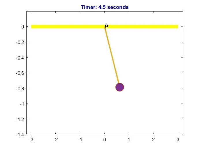
Here "P" is the fixed pivot point. This is the position of bob at t = 4.5 second.
SIMULATION VIDEO:
Youtube link: https://youtu.be/YVyo41dcXLY
FACED CHALLENGE WHILE CODING:
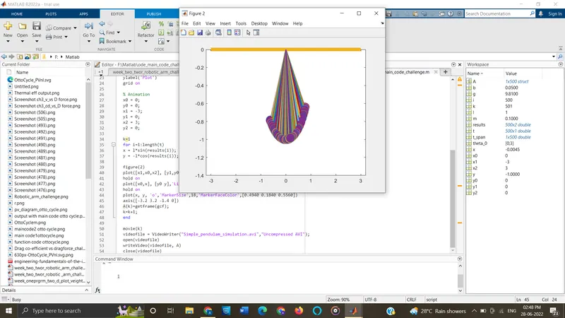
When I first Run the code the bob movement was captured as shown in above figure. Here each frame overlaps one another in the same plot. While I re-verify the code I understand that it is due to the absence of hold off command. So I made equired changes in the code as shown below to overcome this effect (marked in green).
- The code which solves the ODE which represents the equation of motion of a simple pendulum with damping is created by using MATLAB.
- The pendulum motion is simulated and is saved as a video.
- The plot to show the variation in angular displacement and angular velocity with respect to time is created.