Project 2 - Rankine cycle Simulator

PROGRAM: RANKINE CYCLE SIMULATOR

AIM:

To write a program which,

• Create a Rankine Cycle Simulator using MATLAB and calculate net work output & back work ratio for the given condition.
• Calculate the state points of the Rankine Cycle (any type of your choice) based on user inputs.
• Plot the corresponding T-s and h-s plots for the given set of inputs.

OBJECTIVE:

• Understand the working of a rankine cycle simulator.
• Explain the working of Rankine cycle using T-s and h-s diagram.
• Understand the MATLAB coding to find the state points and how the thermodynamic relation helps to get the points inbetween the state variables.

THEORY:

A Rankine cycle power system is a heat engine converting thermal energy into work. Similar to the vapor compression heat pump, it comprises four main components: a boiler (sometimes called evaporator), a turbine, a condenser and a pump.

The working fluid in a low-pressure slightly subcooled liquid state is brought to high pressure by the pump. The pump consumes power. The high-pressure liquid enters the boiler, where it is heated-up, vaporized and potentially heated again to leave the boiler in superheated vapor state. Thermal power must be supplied to the boiler by an external heat source. At the outlet of the boiler, the high-pressure vapor enters the turbine where it is expanded down to the low pressure. The turbine delivers mechanical power.

As a function of the nature of the working fluid and turbine inlet state, the fluid at the end of the expansion can be in superheated vapor state or in two-phase state. At the outlet of the turbine, the fluid enters the condenser where it is condensed to liquid state and, then, slightly subcooled. Thermal power rejected at the condenser is dumped into a heat sink. The low-pressure subcooled liquid enters the pump again.
The net power delivered by the Rankine cycle system is the power delivered by the turbine minus that consumed by the pump.

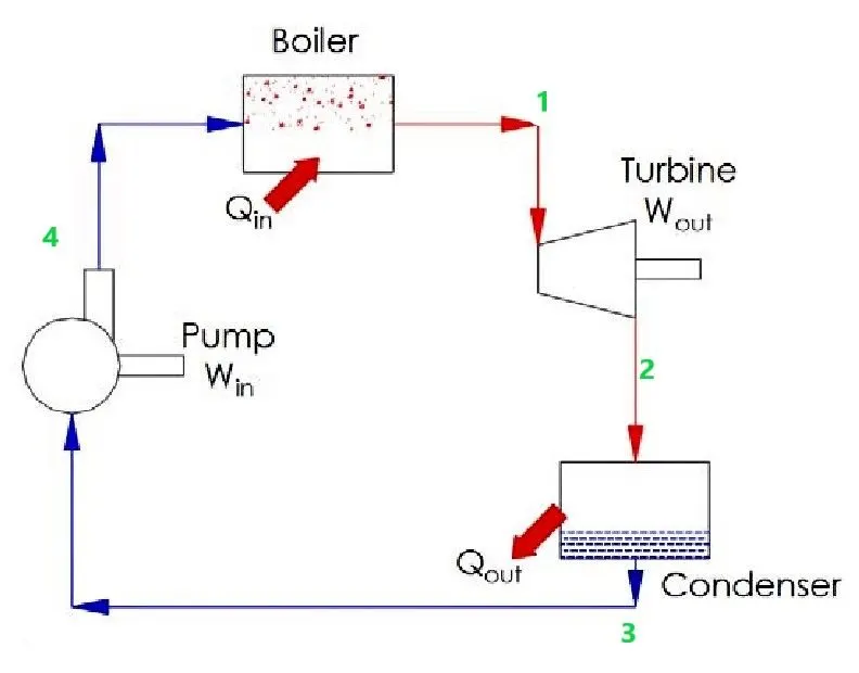
• Process 1-2 Isentropic expansion : The vapor is expanded in the turbine, thus producing work which may be converted to electricity. In practice, the expansion is limited by the temperature of the cooling medium and by the erosion of the turbine blades by liquid entrainment in the vapor stream as the process moves further into the two-phase region. Exit vapor qualities should be greater than 90%.
• Process 2-3 Isobaric Heat Rejection : The vapor-liquid mixture leaving the turbine (2) is condensed at low pressure, usually in a surface condenser using cooling water. In well designed and maintained condensers, the pressure of the vapor is well below atmospheric pressure, approaching the saturation pressure of the operating fluid at the cooling water temperature.
  
  
• Process 3-4 Isentropic Compression : The pressure of the condensate is raised in the feed pump. Because of the low specific volume of liquids, the pump work is relatively small and often neglected in thermodynamic calculations.
  
  
• Process 4-1 Isobaric Heat Addition : High pressure liquid enters the boiler from the feed pump (4) and is heated to the saturation temperature (4s). Further addition of energy causes evaporation of the liquid until it is fully converted to saturated steam (1s). Then it will be superheated to state 1.
  
  
• XSteam:

  XSteam is an implementation of the IAPWS IF97 standard formulation. It provides accurate data for water and steam and mixtures of water and steam properties from 0 - 1000 bar and from 0 - 2000°C. It is available for MATLAB, Excel, OpenOffice, and as a DLL.

  Provided thermodynamic properties are:

  • Temperature
  • Pressure
  • Enthalpy
  • Specific volume
  • Density
  • Specific entropy
  • Specific internal energy
  • Specific isobaric heat capacity
  • Specific isochoric heat capacity
  • Speed of sound
  • Viscosity
  • Vapour fraction

  All properties can be calculated with the inputs, p and T known, p and h known, h and s known and some with pressure and density known.

  XSteam is a full implementation of the IF-97 formulation including all regions and all backward functions for good calculation speed. The code is speed optimized with pressure and enthalpy as inputs for dynamic simulations.

GOVERNING EQUATION:

Heat addition `(Q_"in" )= h_1-h_4`

Heat rejection `(Q_"out")=h_2-h_3`

Work done by turbine `(W_t)=h_1-h_2`

Work done by pump `(W_p)=h_4-h_3`

Net work output `(W_"net")=W_t-W_p`

Thermal efficiency `(eta_"thermal")=W_"net"/Q_"in"`

Back work ratio `(BWR) =W_p/W_t`

Specific steam consumption `(SSC)=3600/W_"net"`

But the work done by pump is negligible, therefore

Steam rate or Specific steam consumption = `3600/W_t`

Where,

h1 = Enthalpy at turbine inlet

h2 = Enthalpy at turbine outlet

h3 = Enthalpy at pump inlet

h4 = Enthalpy at pump outlet

CODE:

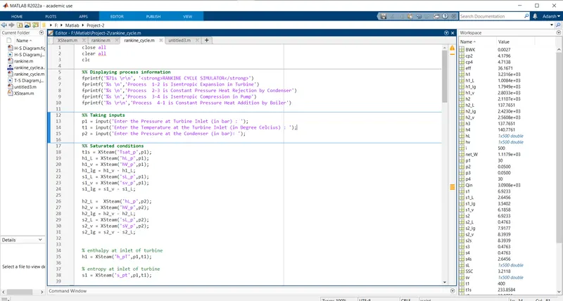
close all
clear all
clc

%% Displaying process information
fprintf('%71s rn', 'RANKINE CYCLE SIMULATOR')
fprintf('%s n','Process  1-2 is Isentropic Expansion in Turbine')
fprintf('%s n','Process  2-3 is Constant Pressure Heat Rejection by Condenser')
fprintf('%s n','Process  3-4 is Isentropic Compression in Pump')
fprintf('%s rn','Process  4-1 is Constant Pressure Heat Addition by Boiler')

%% Taking inputs
p1 = input('Enter the Pressure at Turbine Inlet (in bar) : ');
t1 = input('Enter the Temperature at the Turbine Inlet (in Degree Celcius) : ');
p2 = input('Enter the Pressure at the Condenser (in bar): ');

%% Saturated conditions
t1s = XSteam('Tsat_p',p1);
h1_L = XSteam('hL_p',p1);
h1_v = XSteam('hV_p',p1);
h1_lg = h1_v - h1_L;
s1_L = XSteam('sL_p',p1);
s1_v = XSteam('sv_p',p1);
s1_lg = s1_v - s1_L;

h2_L =  XSteam('hL_p',p2);
h2_v = XSteam('hV_p',p2);
h2_lg = h2_v - h2_L;
s2_L = XSteam('sL_p',p2);
s2_v = XSteam('sV_p',p2);
s2_lg = s2_v - s2_L;


% enthalpy at inlet of turbine
h1 = XSteam('h_pT',p1,t1);

% entropy at inlet of turbine
s1 = XSteam('s_pt',p1,t1);

% conditions at inlet of condenser
% entropy
s2 = s1;
t2s = XSteam('Tsat_p',p2);
s2s = XSteam('sv_p',p2);
cp2 = XSteam('CpL_p',p2);

% dry fraction
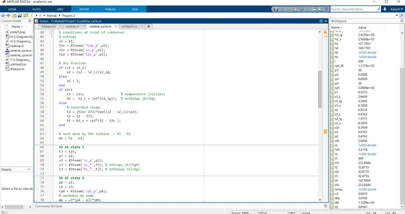
if (s2 < s2_v)
    x2 = (s2 - s2_L)/s2_lg;
else
    x2 = 1;
end
if x2<1
    t2 = t2s;                   % temperature (celsius)
    h2 =  h2_L + (x2*(h2_lg));  % enthalpy (kJ/kg)
else
    % saturated steam
    t2 = (t2s+ 273)*exp((s2 - s2_v)/cp2);
    t2 = t2 - 273;
    h2 = h2_v + cp2*(t2 - t2s );
end

% work done by the turbine  = h1 - h2 
Wt = h1 - h2;

%% At state 3
t3 = t2s;
p3 = p2;
v3 = XSteam('vL_p',p3);
s3 = XSteam('sL_T',t3); % entropy (kJ/kgK)
h3 = XSteam('hL_T',t3); % enthalpy (kJ/kg)

%% At state 4
p4 = p1;
s4 = s3;
cp4 = XSteam('cpl_p',p4);
% workdone by pump
Wp = v3*(p4 - p3)*100;
h4 = Wp + h3;
t4s = XSteam('Tsat_p',p4);  
s4s = XSteam('sL_p',p4);
t4 = t1s/exp((s4s-s4)/cp4);

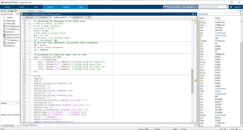
%% calculating the efficiency of the rankin cycle
% work by turbine - Wt Kj/kg
% work by pump -Wp kj/Kg
% net work = Wt- Wp
net_W = Wt-Wp;
% heat added to system = h1-h4
Qin = h1 - h4;
% efficiency = net work/heat added
eff = (net_W/Qin)* 100;
%% back work ratio (BWK=Wp/Wt) and specific steam consumption
BWK = Wp/Wt;
% specific steam consumption
SSC = 3600/Wt;

%% calculating the liquid and vapour line for water
temp = linspace(1,374,500);
for i = 1:length(temp)
    hL(i) = XSteam('hL_T',temp(i)); % enthalpy along the liquid line
    hv(i) = XSteam('hv_T', temp(i)); % enthapy along vapour line
    sL(i) = XSteam('sL_T',temp(i));  % entropy along the liquid line
    sv(i) = XSteam('sv_T',temp(i));  % entropy along vapour line
end

%% T-S 
figure(1)
hold on
plot([s1,s2],[t1,t2],'LineWidth',1.5)
text(s1,t1,' 1')
text(s2,t2,' 2')
plot([s2,s3],[t2,t3],'LineWidth',1.5)
text(s3,t3,' 3')
plot([s3,s4],[t3,t4],'LineWidth',1.5)
text(s4,t4,' 4')
plot([s4,s4s],[t4,t4s],'LineWidth',1.5,'color','r')
text(s4s,t4s,'4s')
plot([s4s,s1_v],[t4s,t1s],'LineWidth',1.5,'color','r')
text(s1_v,t1s,'1s')
plot([s1_v,s1],[t1s,t1],'LineWidth',1.5,'color','r')
plot(sL,temp,'g','LineStyle','--','LineWidth',1.5)
plot(sv,temp,'g','LineStyle','--','LineWidth',1.5)
title('T - S Diagram')
xlabel('Entropy (kJ/kg-K)')
ylabel('Temperature (Degree Celcius)')
grid on
legend('Isentropic expansion','Isobaric heat rejection','Isentropic compression','Isobaric heat addition','','','Saturation curve')
axis([0 12 0 500])

%% H-S plot 
figure(2)
hold on
plot([s1,s2],[h1,h2],'LineWidth',1.5)
text(s1,h1,' 1')
text(s2,h2,' 2')

plot([s2,s3],[h2,h3],'LineWidth',1.5)
text(s3,h3,'   3')
plot([s3,s4],[h3,h4],'LineWidth',1.5)
text(s4,h4,'4')
plot([s4,s1],[h4,h1],'LineWidth',1.5,'color','r')
plot(sL,hL,'g','LineStyle','--','LineWidth',1.5)
plot(sv,hv,'g','LineStyle','--','LineWidth',1.5)
title('H - S Diagram')
xlabel('Entropy (kJ/kg-K)')
ylabel('Enthalpy (kJ/kg)')
grid on
legend('Isentropic expansion','Isobaric heat rejection','Isentropic compression','Isobaric heat addition','Saturation curve')
axis([0 12 0 4000])

%% Displaying result
fprintf('n %62s n', 'RESULTS')
fprintf('%-60s %31s n', 'At State Point 1:','At State Point 4:' )
fprintf('%s %.2f %s %64s %.2f %s n','P1 is :',p1,'Bar','P4 is :',p4,'Bar')
fprintf('%s %.2f %s %55s %.2f %s n','T1 is :',t1,'Deg Celcius','T4 is :',t4,'Deg Celcius')
fprintf('%s %.2f %s %60s %.2f %s n','H1 is :',h1,'kJ/kg','H4 is :',h4,'kJ/kg')
fprintf('%s %.2f %s %62s %.2f %s rn','S1 is :',s1,'kJ/kg-K','S4  is :',s4,'kJ/kg-K')

fprintf('%-60s %22s %.2f %s n', 'At State Point 2:','Wt is : ',Wt,'kJ/kg')
fprintf('%s %.2f %s %65s %.2f %s n','P2 is : ',p2,'Bar','Wp is : ',Wp,'kJ/kg')
fprintf('%s %.2f %s %58s %.2f %s n','T2 is : ',t2,'Deg Celcius','Wnet is : ',net_W,'kJ/kg')
fprintf('%s %.2f %s %64s %.2f %s n','H2 is : ',h2,'kJ/kg','Ntherm is : ',eff,'Percent')
fprintf('%s %.2f %s %64s %.2f %s n','S2 is : ',s2,'kJ/kg-K','S.S.C is : ',SSC,'kJ/kg-K')
fprintf('%s %.2f %82s %f rn','X2 is : ',x2,'Back Work Ratio is : ',BWK)

fprintf('%-60s n', 'At State Point 3:')
fprintf('%s %.2f %s n','P3 is :',p3,'Bar')
fprintf('%s %.2f %s n','T3 is :',t3,'Deg Celcius')
fprintf('%s %.2f %s n','H3 is :',h3,'kJ/kg')
fprintf('%s %.2f %s n','S3 is :',s3,'kJ/kg-K')

Explanation:

Note: Here we uses XSteam function to get steam data.

Taken Input condition:

Turbine Inlet temperature = 400° C

Turbine Inlet Pressure = 30 bars

Turbine Outlet Pressure = 0.05 bars = Condenser Inlet Pressure

• First of all, we display the Rankine cycle processes using the fprintf() command.
  
  %% Displaying process information
  fprintf('%71s rn', 'RANKINE CYCLE SIMULATOR')
  fprintf('%s n','Process 1-2 is Isentropic Expansion in Turbine')
  fprintf('%s n','Process 2-3 is Constant Pressure Heat Rejection by Condenser')
  fprintf('%s n','Process 3-4 is Isentropic Compression in Pump')
  fprintf('%s rn','Process 4-1 is Constant Pressure Heat Addition by Boiler')
• Then using the input() command, we take the values for Turbine inlet pressure, Turbine inlet temperature ,Turbine outlet pressure as 30 bar, 400 Deg Celsius and 0.05 bar respectively.
  
  %% Taking inputs

  p1 = input('Enter the Pressure at Turbine Inlet (in bar) : ');

  t1 = input('Enter the Temperature at the Turbine Inlet (in Degree Celcius) : ');SSS

  p2 = input('Enter the Pressure at the Condenser (in bar): ');
• Put XSteam.m file in same directory and call the XSteam function with suitable arguments to find the values of enthalpy, entropy for state 1 and 2. Also finding the work done by turbine as per equation. We also check the dryness fraction at state point 2 to know whether the outlet from turbine is complete steam or not (or liquid + vapour).
  
  %% Saturated conditions

  t1s = XSteam('Tsat_p',p1);

  h1_L = XSteam('hL_p',p1);

  h1_v = XSteam('hV_p',p1);

  h1_lg = h1_v - h1_L;

  s1_L = XSteam('sL_p',p1);

  s1_v = XSteam('sv_p',p1);

  s1_lg = s1_v - s1_L;

  h2_L = XSteam('hL_p',p2);

  h2_v = XSteam('hV_p',p2);

  h2_lg = h2_v - h2_L;

  s2_L = XSteam('sL_p',p2);

  s2_v = XSteam('sV_p',p2);

  s2_lg = s2_v - s2_L;

  % enthalpy at inlet of turbine

  h1 = XSteam('h_pT',p1,t1);

  % entropy at inlet of turbine

  s1 = XSteam('s_pt',p1,t1);

  % conditions at inlet of condenser

  % entropy

  s2 = s1;

  t2s = XSteam('Tsat_p',p2);

  s2s = XSteam('sv_p',p2);

  cp2 = XSteam('CpL_p',p2);

  % dry fraction

  if (s2 < s2_v)

  x2 = (s2 - s2_L)/s2_lg;

  else

  x2 = 1;

  end

  if x2<1

  t2 = t2s; % temperature (celsius)

  h2 = h2_L + (x2*(h2_lg)); % enthalpy (kJ/kg)

  else

  % saturated steam

  t2 = (t2s+ 273)*exp((s2 - s2_v)/cp2);

  t2 = t2 - 273;

  h2 = h2_v + cp2*(t2 - t2s );

  end

  % work done by the turbine = h1 - h2

  Wt = h1 - h2;
• Similarly, We use XSteam function to get variables at state point 3 and 4. (T, S, H). Also find out the pump work by using equations.
  
  %% At state 3

  t3 = t2s;

  p3 = p2;

  v3 = XSteam('vL_p',p3);

  s3 = XSteam('sL_T',t3); % entropy (kJ/kgK)

  h3 = XSteam('hL_T',t3); % enthalpy (kJ/kg)
  
  

  %% At state 4

  p4 = p1;

  s4 = s3;

  cp4 = XSteam('cpl_p',p4);
  

  % workdone by pump

  Wp = v3*(p4 - p3)*100;

  h4 = Wp + h3;

  t4s = XSteam('Tsat_p',p4);

  s4s = XSteam('sL_p',p4);

  t4 = t1s/exp((s4s-s4)/cp4);
• After that, we give code to find out Net work, Heat addition, Efficiency, Back work ration and Specific steam consumption.
  
  %% calculating the efficiency of the rankin cycle

  % work by turbine - Wt Kj/kg

  % work by pump -Wp kj/Kg

  % net work = Wt- Wp

  net_W = Wt-Wp;

  % heat added to system = h1-h4

  Qin = h1 - h4;

  % efficiency = net work/heat added

  eff = (net_W/Qin)* 100;

  %% back work ratio (BWK=Wp/Wt) and specific steam consumption

  BWK = Wp/Wt;

  % specific steam consumption

  SSC = 3600/Wt;
• By using a a for loop, we find the values of enthalpy and entropy of water at saturated liquid and vapour line for a temperature range between 1 and 374. We use these values for plotting saturation curve in T-S and H-S diagram.
  
  %% calculating the liquid and vapour line for water
  temp = linspace(1,374,500);
  for i = 1:length(temp)
  hL(i) = XSteam('hL_T',temp(i)); % enthalpy along the liquid line
  hv(i) = XSteam('hv_T', temp(i)); % enthapy along vapour line
  sL(i) = XSteam('sL_T',temp(i)); % entropy along the liquid line
  sv(i) = XSteam('sv_T',temp(i)); % entropy along vapour line
  end
• By using the plot command, we plot T-S and H-S diagram as figure1 and figure2 respectively as shown in the code given in the code section of this report. This plotting is done by joining each state point. The plot is given with x, y labels , legends, proper heading (by using title command) and grids for better understanding. By using text() command the state point is also mentioned in the graph.
  
  
• At last, the Results are get arranged by using fprintf() command as shown in the code given in the code section of this report. The P, T, H, S at each state point is displayed. Also Wp, Wt, Wnet, Steam rate and Back work ratio also displayed using fprintf() command.
  All datas are properly arranged by giving providing spaces using the command code.
  
  

OUTPUT:

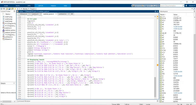
• Code:
  
  
  
  
  
  
• T-S Diagram:
  
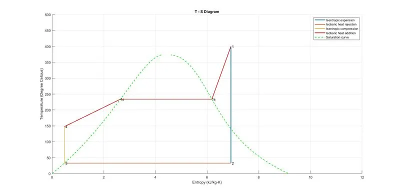
  Here pump and turbine works isentropically. The isentropic expansion of superheated steam in the turbine is Process 1-2. After expansion the state point 2 is inside the saturation dome, that is the point 2 contain working fluid in both liquid and vapour state. After isentropic compression in pump(3-4), the high pressure water enters the boiler (at 4) which converts completely into steam at 4s. Then it superheated to a state point 1.
  
  
• H-S Diagram:
  
  
  
  
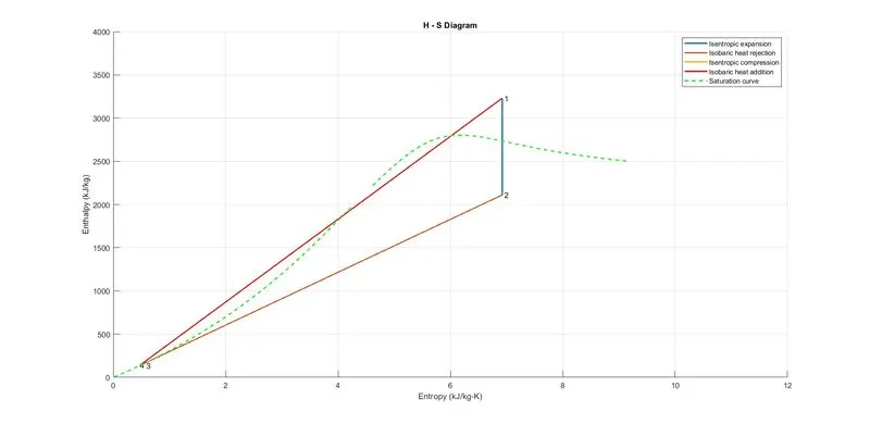
• Command window:
  
  

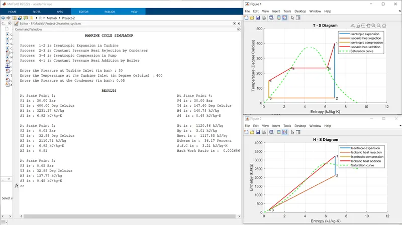
RANKINE CYCLE SIMULATOR

Process 1-2 is Isentropic Expansion in Turbine
Process 2-3 is Constant Pressure Heat Rejection by Condenser
Process 3-4 is Isentropic Compression in Pump
Process 4-1 is Constant Pressure Heat Addition by Boiler

Enter the Pressure at Turbine Inlet (in bar) : 30
Enter the Temperature at the Turbine Inlet (in Degree Celcius) : 400
Enter the Pressure at the Condenser (in bar): 0.05

RESULTS
At State Point 1: At State Point 4:
P1 is : 30.00 Bar P4 is : 30.00 Bar
T1 is : 400.00 Deg Celcius T4 is : 147.60 Deg Celcius
H1 is : 3231.57 kJ/kg H4 is : 140.78 kJ/kg
S1 is : 6.92 kJ/kg-K S4 is : 0.48 kJ/kg-K

At State Point 2: Wt is : 1120.86 kJ/kg
P2 is : 0.05 Bar Wp is : 3.01 kJ/kg
T2 is : 32.88 Deg Celcius Wnet is : 1117.85 kJ/kg
H2 is : 2110.71 kJ/kg Ntherm is : 36.17 Percent
S2 is : 6.92 kJ/kg-K S.S.C is : 3.21 kJ/kg-K
X2 is : 0.81 Back Work Ratio is : 0.002686

At State Point 3:
P3 is : 0.05 Bar
T3 is : 32.88 Deg Celcius
H3 is : 137.77 kJ/kg
S3 is : 0.48 kJ/kg-K

where,
P, T, H, S followed by a number indicate pressure, temperature, enthalpy and entropy at each state point. The number indicate the state point.

X2 - Dryness fraction at state 2

Wp - Pump work

Wt - Turbine work

Wnet - Net work

Ntherm - Thermal efficiency

S.S.C - Specific steam consumption

RESULT:

• Created a Rankine Cycle Simulator using MATLAB and calculate net work output & back work ratio for the given condition by using code.
  Net work output = 1117.85 kJ/kg
  Back work ratio = 0.002686
  
  
• Marked the state points of the Rankine Cycle (any type of your choice) based on user inputs by using code.
  
  
• The T-s and h-s plots were plotted for the given set of inputs.

CONCLUSION:

• We can understand and explain the working of a rankine cycle by using T-S and H-S diagram.

• Rankine cycle is a power generating cycle. Superheating increase the thermal efficiency of cycle.

• Understand the MATLAB coding to find the state points and how the thermodynamic relation helps to get the points in-between the state variables.

REFERENCE:

• https://in.mathworks.com/matlabcentral/fileexchange/9817-x-steam-thermodynamic-properties-of-water-and-steam
• https://www.thermopedia.com/content/1072/
• https://www.sciencedirect.com/topics/earth-and-planetary-sciences/rankine-cycle
• Basic and Applied Thermodynamics, P K Nag.