Global Maxima of a staligmite function
Aim - To write a code in MATLAB to optimise the staligmite function and find the Global Maxima of the function.
Theory:-
A stalagmite is a type of rock formation that rises from the floor of a cave due to the accumulation of material deposited on the floor from celing drippings. Stalagmites are typically composed of calcium carbonate, but may consist of lava, mud, peat, pitch, sand, sinter and amberat. The rock formation of celing drippings is known as Stalactite.
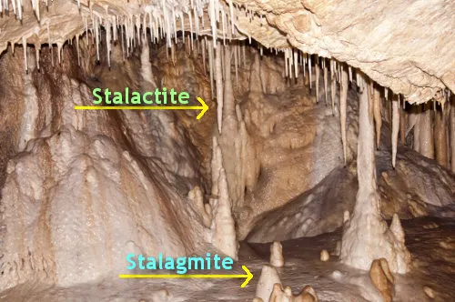
A stalagmite function generally refers to the function with which we are generating values over a stalagmite kind of surface for finding out the local and global maxima and minima of that particular given function. For this in Matlab we are using a method called 'Optimization'.
The peaks of the stalagmite surface are known as local maxima while the highest peak is known as the global maxima.
Genetic Algorithim:-
A genetic algorithm (GA) is a method for solving both constrained and unconstrained optimization problems based on a natural selection process that mimics biological evolution. The algorithm repeatedly modifies a population of individual solutions. At each step, the genetic algorithm randomly selects individuals from the current population and uses them as parents to produce the children for the next generation. Over successive generations, the population "evolves" toward an optimal solution.
We can apply the genetic algorithm to solve problems that are not well suited for standard optimization algorithms, including problems in which the objective function is discontinuous, nondifferentiable, stochastic, or highly nonlinear.
The genetic algorithm finds the minima of a function. However we can modify the function and find maxima of the function using the same.
Syntax for Genetic Algorithm (ga)
x = ga(fun,nvars) finds a local unconstrained minimum x to the objective function, fun and nvars is the dimension (number of design variables) of fun.
x = ga(fun,nvars,A,b) finds a local minimum x to fun, subjected to the linear inequalities A*x ≤ b. ga evaluates the matrix product A*x as if x is transposed (A*x').
x = ga(fun,nvars,A,B,Aeq,Beq) finds a local minimum x to fun, subjected to the linear inequalities Aeq*x = Beq , A*x ≤ b (Set A=[] and B = [] if no linear inequalities exist.) ga evaluates the matrix product Aeq*x as if x is transposed (Aeq*x').
x = ga(fun,nvars,A,B,Aeq,Beq,lb,ub) defines a set of lower and upper bounds on the design variables, 'x' so that a solution is found in the range lb ≤ x ≤ ub. (Set Aeq=[] and Beq = [] if no linear equalities exist.)
x = ga(fun,nvars,A,B,Aeq,Beq,lb,ub,nonlcon) subjects the minimization to the constraints defined in nonlcon. The function nonlcon accepts x and returns vectors C and Ceq, representing the nonlinear inequalities and equalities respectively. ga minimizes the fun such that C(x) ≤ 0 and Ceq(x) = 0. (Set lb = [] and ub = [] if no bounds exist.)
x = ga(fun,nvars,A,B,Aeq,Beq,lb,ub,nonlcon,options) minimizes with the default optimization parameters replaced by values in options. (Set nonlcon = [] if no nonlinear constraints exist.) Create options using 'optimoptioms'.
x = ga(fun,nvars,A,B,[],[],lb,ub,nonlcon,IntCon) or x = ga(fun,nvars,A,B,[],[],lb,ub,nonlcon,IntCon,options) requires that the variables listed in IntCon take integer values. When there are integer constraints, ga does not accept linear or nonlinear equality constraints, only inequality constraints.
x = ga(problem) finds the minimum for problem, a structure is described in the problem.
[x,fval] = ga(___) for any previous input arguments, also returns fval, the value of the fitness function at x.
[x,fval,exitflag,output] = ga(___) also returns an exitflag, an integer identifying the reason the algorithm terminated, and output, a structure that contains output from each generation and other information about the performance of the algorithm.
[x,fval,exitflag,output,population,score] = ga(___) also returns a matrix population, whose rows are the final population, and a vector scores, the scores of the final population.
Function
`f = (f1x*f1y*f2x*f2y)`
`f1x = (sin((5.1*pi*x) + 0.5))^6`
`f1y = (sin((5.1*pi*y) + 0.5))^6`
`f2x = exp((-4*(log(2)))*((x-0.0667)^2)/0.64)`
`f2y = exp((-4*(log(2)))*((y-0.0667)^2)/0.64)`
Code:-
Function for stalagmite
function f = stalagmite(input_vec)

x = input_vec(1);
y = input_vec(2);

f1x = (sin((5.1*pi*x) + 0.5))^6;
f1y = (sin((5.1*pi*y) + 0.5))^6;
f2x = exp((-4*(log(2)))*((x-0.0667)^2)/0.64);
f2y = exp((-4*(log(2)))*((y-0.0667)^2)/0.64);

f = -(f1x*f1y*f2x*f2y);

% The ga command solves for the minima, in this case we want to find the
% maxima. Hence we use the negative sign operator.
Function to get stalagmite
function f = get_stalagmite(x,y)

% Creating 2D mesh
[xx,yy] = meshgrid(x,y);

% Evaluating the function
for i = 1:length(xx)
    for j = 1:length(yy)
        input_vec(1) = xx(i,j);
        input_vec(2) = yy(i,j);

       f(i,j) = -stalagmite(input_vec);
% Since the function output is a stalactites and the we need to find for
% stalagmites we use negative sign.

    end
end
Main program
clear all
close all
clc

% Defining Inputs
x = linspace(0,0.6,150);
y = linspace(0,0.6,150);
num_cases = 50;

% Calling the function
f = get_stalagmite(x,y);

tic
% Study 1 - Statistical behaviour
for i = 1:num_cases
    [inp,fopt(i)] = ga(@stalagmite,2);
    xopt(i) = inp(1);
    yopt(i) = inp(2);
end

% The fopt generated from the ga command solves for the minimum points, to
% find the maxima we use negative sign operator.

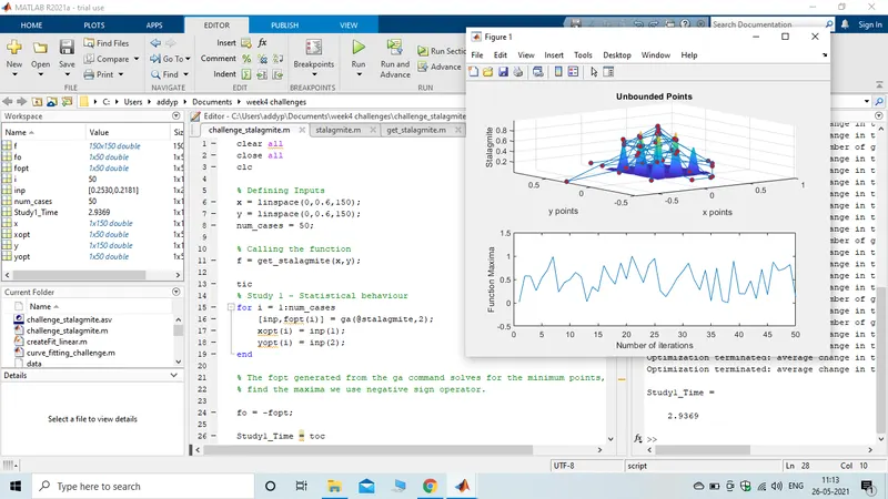
fo = -fopt;

Study1_Time = toc

figure(1)
subplot(2,1,1)
surfc(x,y,f)
shading interp
xlabel('x points')
ylabel('y points')
zlabel('Stalagmite')
title('Unbounded Points')
hold on
plot3(xopt,yopt,fo,'marker','o','markersize',5,'markerfacecolor','r')
subplot(2,1,2)
plot(fo)
axis([0 50 -0.5 1.5])
xlabel('Number of iterations')
ylabel('Function Maxima')


tic
% Study 2 - Statistical behaviour with upper and lower bounds

for i = 1:num_cases
    [inp,fopt(i)] = ga(@stalagmite,2,[],[],[],[],[0 0],[0.6 0.6]);
    % x and y are matrices having value from 0 to 0.6, hence lower and
    % upper bounds [0 0] and [0.6 0.6] respectively.
    xopt(i) = inp(1);
    yopt(i) = inp(2);
end

% The fopt generated from the ga command solves for the minimum points, to
% find the maxima we use negative sign operator.

fo = -fopt;


Study2_Time = toc

figure(2)
subplot(2,1,1)
surfc(x,y,f)
shading interp
xlabel('x points')
ylabel('y points')
zlabel('Stalagmite')
title('Bounded Points')
hold on
plot3(xopt,yopt,fo,'marker','o','markersize',5,'markerfacecolor','r')
subplot(2,1,2)
plot(fo)
axis([0 50 0.5 1.5])
xlabel('Number of iterations')
ylabel('Function Maxima')


tic
% Study 3 - Statistical Behaviour with upper and lower bounds with more
% iterations

options = optimoptions('ga')
options = optimoptions(options,'PopulationSize',150)

for i = 1:num_cases
    [inputs,fopt(i)] = ga(@stalagmite,2,[],[],[],[],[0 0],[0.1 0.1],[],[],options);
    % From study 2 we can observe that the maxima of the function lies
    % between x(0,0.1) and y(0,0.1). Therefore defining the search space
    % lower bound [0 0] and upper bound [0.1 0.1]. Also iterating for more
    % number of time so that we get the global maxima and not local maxima
    xopt(i) = inputs(1);
    yopt(i) = inputs(2);
end

% The fopt generated from the ga command solves for the minimum points, to
% find the maxima we use negative sign operator.

fo = -fopt;

Study3_time = toc

figure(3)
subplot(2,1,1)
surfc(x, y, f)
shading interp
xlabel('x points')
ylabel('y points')
zlabel('Stalagmite')
title('Maxima')
hold on
plot3(xopt, yopt, fo,'marker','o','markersize',5,'markerfacecolor','r')
axis([0 0.6 0 0.6 0 1.2])
title('Global Maxima')
subplot(2,1,2)
plot(fo)
axis([0 50 0 2])
xlabel('Number of Iterations')
ylabel('Function Maxima')
Outputs:-
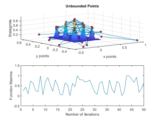
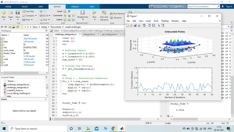
Study 1 - Unbounded Points
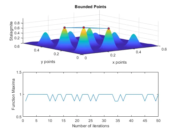
Study 2 - Unbounded Points
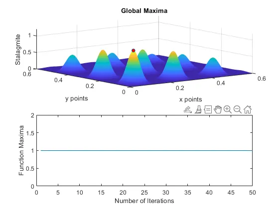
Study 3 - Global Maxima
Errors Faced:-
The fopt values we are getting are negative, this is due to the changes we made in the functions to get the maxima instead of minima.
This is resolved by introducing a variable which is negative of fopt
Explaination of code:-
We start the code intially by writing the function given to us. We have to find f(x,y) which is the product of functions f1x,f1y,f2x,f2y. Since 2 variables are involved while taking the product the number of rows and column must match.
For this we write another function where we get the stalagmite. In this the meshgrid command is used get xx and yy and these are used along with the nested for loop to get the stalagmite function. Negative sign operator is used so that the function finds the maxima instead of minima.
In the main program the input arrays are mentioned. Variable num_cases is introduced which will determine the number of iterations. The function get_stalagmite is called which will be ploted along the z axis.
Study 1 is performed to check the statistical behaviour of the function. For loop is runned along all the number of iterations. The ga (genetic algorith) command is used to get the x,y and f values for all the iterations these values are know as the optimum values described as xopt, yopt and fopt. The fopt value we get is negative since we are finding the maxima of stalagmite function we need the positive value, so we multiple fopt with negative sign operator. tic and toc command are used to get the running time of the Study 1.
For plotting we use the subplot command as we have to plot the stalagmite function and we have to plot the fopt points on the function as well as we have to observe the how the function maxima varies along the iterations. As the function is ploted using surfc command shading interp command is use to get a smooth look on the function. In the plots we observe that the points for the function maxima are all over the function as well as outside the function. Hence we conduct Study 2.
In Study 2 we mention the upper and lower bounds in the ga command, this allows all the maxima point to lie in the function and not outside. But still we have not found the Global Maxima. So we conduct Study 3.
In Study 3 we introduce the command option and optimoptions with the help of this we can iterate the function for more number of times so that with more iterations our chances of finding the global maxima are more. Also we can figure out around where the Global maxima is in Study 2. Hence by shrinking the bounds we can get more accurate result.
Conclusion : Hence we have found the Global Maxima of the function given. The time required for the next study is always greater than the previous. This is because the next study is going for more accurate results. For accurate results the number iterations must be greater. By defining the search space more specificaly we can find the output accurately. The genetic algorithm command is used to find the minima of a function but with some modification we can also find the maxima using (ga) function.
Refrences:
https://in.mathworks.com/help/gads/how-the-genetic-algorithm-works.html
https://in.mathworks.com/help/gads/ga.html#mw_a07ddf7d-face-4243-a656-f1528b592de0