Second order ODEs

Objective - To write a program that solves ODE which represents the equation of motion of a simple pendulum with damping.

Theory:-

A pendulum is a weight suspended from a pivot so that it can swing freely. When a pendulum is displaced sideways from its resting position (equilibrium position) it is subjected to a restoring force due to gravity that will accelerate it back toward the equilibrium position. When released, the restoring force acting on the pendulum's mass causes it to oscillate about the equilibrium position, swinging back and forth. While oscillationg back and forth the pendulum experiences some resistances like air resistance or friction which makes the pendulum lose its amplitude periodically. Hence after a time coming to a complete rest. This phenomenon is known as damping.

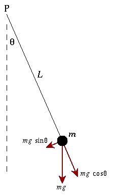
'`theta`' is the angle made by the string of the pendulum with respect to the resting position. This is the angular displacement.

's' is the arc length covered by the pendulum from equilibrium position, `s=theta*L`

'b' is the damping coefficient

'L' is the length of the pendulum

'm' is the mass of the pendulum

'g' is the gravity

Let the force acting on the pendulum be F

`therefore` its x and y component will be Fx = `m*g*sintheta`, Fy = `m*g*costheta`

A restoring force acts on the pendulum to bring back to its equilibrium position.

The restoring force can be given as Fr = `-m*g*sintheta`

`m*(d^2s)/dt^2 = m*L*(d^2theta)/dt^2 = -m*g*sintheta`

` m*(d^2theta)/dt^2 = -m*g/L*sintheta`

The Damping force can be given as, Fd = `-b*v` ...[where '`v`' is the angular velocity]

`m*(d^2 theta)/dt^2 = -b*(d theta)/dt`

`sum`Force = Fr + Fd

`m*(d^2 theta)/dt^2 = -b*(d theta)/dt -m*g/L *sintheta`

`therefore (d^2 theta)/dt^2 + b/m*(d theta)/dt + g/L *sintheta = 0`

Equation :-

`(d^2theta)/dt^2+b/m*(d theta)/dt+g/L*sintheta=0`

Further solving the equation,

Let `theta` = `theta1`

`rArr` `(d theta)/dt = (d theta1)/dt` = `theta2` ...(eq.1)

`rArr` `(d^2theta)/dt^2` = `(d^2theta1)/dt^2` = `(d theta2)/dt` ...(eq.2)

Substituting (eq.1) & (eq.2) in the formula given, we get

`(d theta2)/dt + b/m*theta2 + g/L*sintheta1 = 0`

`therefore (d theta2)/dt = -b/m*theta2 -g/L*sintheta1` ...(eq.3)

Program :-

% Program to solve an ODE which represents the equation of motion of a
% simple pendulum with damping

clear all
close all
clc

% Provided Data
g = 9.81;                  % gravity in m/s^2
L = 1;                     % Length of pendulum in m
m = 1;                     % Mass of pendulum in kg
b = 0.05;                  % Damping Coefficent

% Initial condition, when t = 0
% Angular Displacement, d in rad 
d = 0;
% Angular Velocity, v in rad/s
v = 3;
% Array of initial angular displacement and angular velocity, d_v
d_v = [0;3];

% Time span, t_span in sec
t_span = linspace(0,20,500);

% Solving ODE
[t,results] = ode45(@(t,theta)ode_fun(t,theta,b,g,L,m),t_span,d_v);

% Plotting
figure(1)
plot(t,results(:,1),'color','b')
hold on
plot(t,results(:,2),'color','r')
grid on
axis([0 20 -4 4])
legend('Angular Displacement', 'Angular Velocity')
xlabel('Time Span')
ylabel('Damping Oscillations')
title('Motion of Pendulum')


% Animation for motion of the pendulum

% Angle created by the pendulum is the angular displacement at every time
% interval

angle = results(:,1);

ct=1;
for i = 1:length(angle)
    THETA = angle(i);
    
    figure(2)
    
    % Coordinates where pendulum is attached
    x0 = 0;
    y0 = 0;
    
    % Coordinates where bob is travelling
    x1 = L*sin(THETA);
    y1 = -L*cos(THETA);
    % y1 is negative because the pendulum we are programing for hangs 
    % below the pivot point and cos of negative values is always positive.
    
    
   % Plotting all the points to get an animation video
   plot([x0 x1],[y0 y1],'linewidth',1,'color','black')
   hold on
   plot(x1,y1,'o','markers',15,'MarkerFaceColor','m')
   plot([0.75 -0.75],[0 0],'linewidth',5,'color','g')
   axis([-1 1 -1.2 0.3])
   grid on
   hold off
   title('Damping Pendulum Motion')
   M(ct)=getframe(gcf);
   pause(0.0003)
   ct=ct+1;   
   
end

movie(M)
videofile = VideoWriter('Pendulum_Motion.avi')
open(videofile)
writeVideo(videofile,M)
close(videofile)

Function used in the program

function [dtheta_dt] = ode_fun(t,theta,b,g,L,m)

theta1 = theta(1);
theta2 = theta(2);
dtheta1_dt = theta2;
dtheta2_dt = -(b/m)*theta2-(g/L)*sin(theta1);
dtheta_dt = [dtheta1_dt;dtheta2_dt];

end

Explaination of Code:

• The code is divided into two parts
• First where the main parametrs like mass, length, gravity, damping coefficient are mentioned. The initial condition of angular displacement and angular velocity is also mentioned here using a column matrix. The time span for which we are going to get the output is also mentioned and 500 intervals of the time span are taken with the help of linspace command.
• The function is the second part of the code, where the second order ODE is simplified to the first order ODE in terms of theta1 and theta2. They are then differentiated forming a column matrix of dtheta_dt
• Using the inbuild command ode45, ODE function is called. The ode45 command requires an ode function, the time span for which the function is going to run and the intial conditions. Solving this gives us the value of the conditions with respect to their time interval. By using this data we can plot the conditions with respect to time.
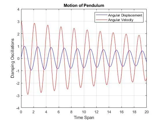
• Hence, angular displacement and angular velocity is plotted with respect to time.
• When the pendulum moves, its one end is fixed and the other end moves to and fro in the same trajectory. For loop is used to get the cordinates of the moving end of pendulum at every interval of time mentioned. Counter (ct) is used to control the iterations of the loop. Plotting the moving coordinates with respect to the fixed end wil display the animation.
• For the animation we need to capture each frame and run them with a small pause to get the video effect. This done by the movie command.
• Grid on command is used in the plot as well as the animation for better understanding of damping.

Output:

Animation:

https://drive.google.com/file/d/1UneJaOOOLQfVl8Ra6JRG25gc5dwU9ng_/view?usp=sharing

Errors faced:

Inverted comma not used in legend to specify the text.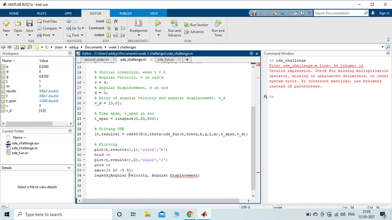

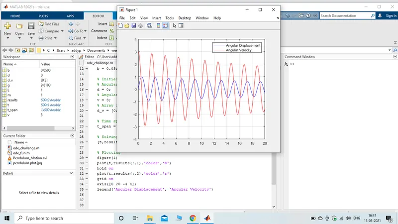
Corrected by using inverted comma in the legend.

Conclusion:

A second order differential equation can be solved using MATLAB. Hence we have animated the motion of a pendulum. From this we can say that the pendulum gradually looses its amplitude (angular displacement) as well as angular velocity with respect to time.