Challenge

Week 4.1 - Genetic Algorithm

SSandeep Raj2 Jul 2022

Aim

To write a code in Matlab to optimise the stalagmite function and find the global maxima of the function.

Genetic Algorithm

The genetic algorithm is a method for solving both constrained and unconstrained optimization problems that is based on natural selection. The genetic algorithm repeatedly modifies a population of individual solutions. At each step, the genetic algorithm selects individuals from the current population to be parents and uses them to produce the children for the next generation. Over successive generations, the population evolves toward an optimal solution. You can apply the genetic algorithm to solve a variety of optimization problems.

This flow chart outlines the main algorithmic steps.

The genetic algorithm differs from a classical, derivative-based, optimization algorithm in two main ways, as summarized in the following table:

Classical Algorithm	Genetic Algorithm
Generates a single point at each iteration. The sequence of points approaches an optimal solution.	Generates a population of points at each iteration. The best point in the population approaches an optimal solution.
Selects the next point in the sequence by a deterministic computation.	Selects the next population by computation which uses random number generators.
Typically converges quickly to a local solution.	Typically takes many function evaluations to converge. May or may not converge to a local or global minimum.

Phases in genetic algorithm:

Initialization of population
Fitness function
Selection
Reproduction 1.) Crossover 2.) Mutation

Steps followed in the code.

The function stalagmite is defined separately. This function is later called into the main program.
Using the linspace command, the inputs for the x and y are defined.
Then, using the meshgrid command, the input vectors are transformed into an array to evaluate function variables and plot 3D surfaces.
Values from the created array is taken as an input to the function stalagmite which is called into the main program.At various x and y, the values of the stalagmite function is generated.
The inbuilt function ga is then used to calculate the maxima value.
num_cases is used to define the number fo iterations and for loop is used to run ga for the number of iterations defined.
ga as an inbuilt function, generally gives the minima value. Therefore inorder to get the maxima value, the stalagmite function is inversed by introducing a negative sign.
The time for the study is calculated using the tic and toc command for each ga loop. Surfc and plot command are used to plot the results.
ga is then run for three case studies.

Stalagmite function

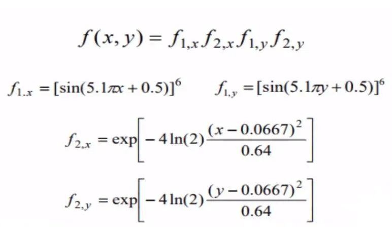
The above governing equation is defined in stalagmite function in MATLAB as:

function [f] = stalagmite(input_vector)

x = input_vector(1);
y = input_vector(2);
f1_x= (sin(5.1*pi*x+ .5))^6;
f1_y= (sin(5.1*pi*y+ .5))^6;
f2_x= exp((-4*log(2))*((x-.0667)^2/.64));
f2_y= exp((-4*log(2))*((y-.0667)^2/.64));

f = -(f1_x*f2_x*f1_y*f2_y)

end

The stalagmite function is called in to the program and run for the results.

clear all 
close all
clc

% Inputs
x = linspace(0,.6,150);
y = linspace(0,.6,150);

% 2D mesh generation
[xx, yy] = meshgrid(x,y);

% Evaluation of the stalagmite function

for i = 1:length(xx);
    for j = 1:length(yy);
        input_vector(1) = xx(i,j);
        input_vector(2) = yy(i,j);
        f(i,j) = stalagmite(input_vector);
    end
end

% Plot - Stalagmite Function
figure(1)
surfc(xx,yy,-f)
shading interp
title('Stalagmite Function')

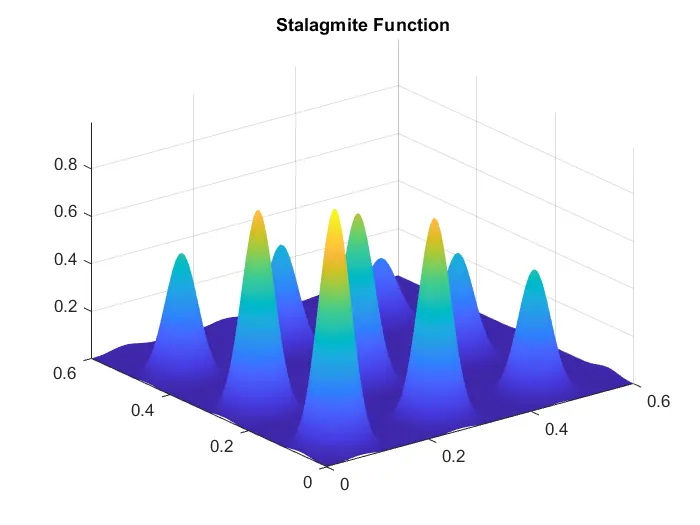
Output Plot

Study 1 - Statistical Behaviour With Unbounded Inputs

For case study 1 no boundary limits are set and therefore the syntax for ga is as follows:

x = ga(fun,nvars) finds a local unconstrained minimum, x, to the objective function. nvars is the dimension (number of design variables) of function.

Here fun is the stalagmite function defined and number of variables is equal to 2.

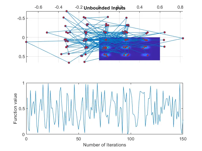
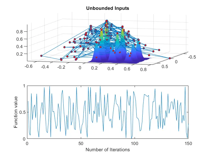
ga is run and the function is evaluated for the defined number of iterations and the results are plotted.

% Study 1 - Satistical Behaviour With Unbounded Inputs

clear all 
close all
clc

% Inputs
x = linspace(0,.6,150);
y = linspace(0,.6,150);

% 2D mesh generation
[xx, yy] = meshgrid(x,y);

% Evaluation of the stalagmite function
for i = 1:length(xx);
    for j = 1:length(yy);
        input_vector(1) = xx(i,j);
        input_vector(2) = yy(i,j);
        f(i,j) = stalagmite(input_vector);
    end
end
% Plot - Stalagmite Function
figure(1)
surfc(xx,yy,-f)
shading interp
title('Stalagmite Function')

num_cases = 150; % ga runs for 150 iterations
tic
for k=1:num_cases
    % using x = ga(fun,nvars) 
    % Objective function is stalagmite and number of variables is 2
    [inputs,f_opt(k)] = ga(@stalagmite,2);
    x_opt(k) = inputs(1);
    y_opt(k) = inputs(2);
end
study_time1= toc 

figure(2)
subplot(2,1,1)
hold on
surfc(xx,yy,-f) % to plot the stalagmite function
shading interp
plot3(x_opt,y_opt,-f_opt,'marker','o','markersize',4,'MarkerFaceColor','r') %plotting the optimum values along the stalagmite 3D curve
title('Unbounded Inputs')
grid on
subplot(2,1,2)
plot(-f_opt)  % plot optf for every iterations
xlabel('Number of Iterations')
ylabel('Function value')

Outplut Plot

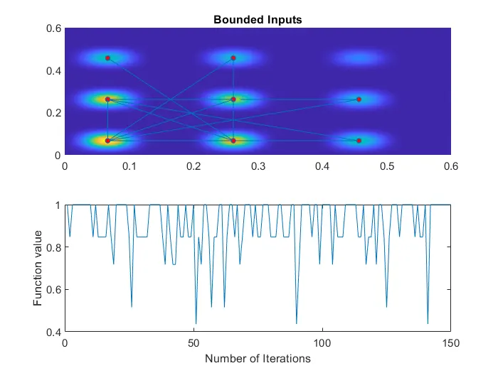
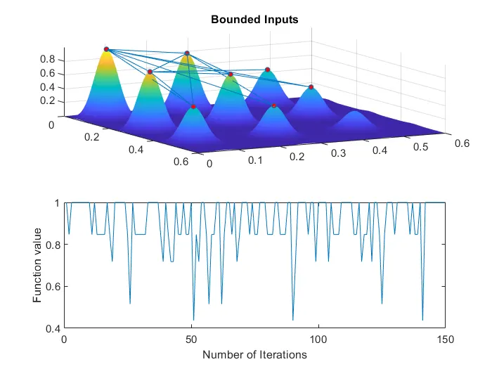
Study 2 - Statistical Behaviour With Bounded Inputs

For this study, as lower bounds and upper bouds are set, the syntax for ga is:

x = ga(fun,nvars,A,b,Aeq,beq,lb,ub) defines a set of lower and upper bounds on the design variables, x, so that a solution is found in the range lb ≤ x ≤ ub. If no linear equalities exist, Aeq and beq are set to [].

% Study 2 - Statistical Behaviour With Bounded Inputs (Lower boundary &
% Upper boundary)

clear all 
close all
clc

% Inputs
x = linspace(0,.6,150);
y = linspace(0,.6,150);

% 2D mesh generation
[xx, yy] = meshgrid(x,y);

% Evaluation of the stalagmite function
for i = 1:length(xx);
    for j = 1:length(yy);
        input_vector(1) = xx(i,j);
        input_vector(2) = yy(i,j);
        f(i,j) = stalagmite(input_vector);
    end
end
% Plot - Stalagmite Function
figure(1)
surfc(xx,yy,-f)
shading interp
title('Stalagmite Function')

num_cases = 150; % ga runs for 150 iterations
tic
for l=1:num_cases
    % using x = ga(fun,nvars,A,b,Aeq,beq,lb,ub) 
    % Objective function is stalagmite and number of variables is 2
    % a,b,Aeq,beq = [], as there are no Linear equalities and inequalities
    % in theis function
    % lb(lower boundary) for x,y in ga are set as [0,0]
    % up(upper boundary) for x,y in ga are set as [1,1]
  
    [inputs,f_opt(l)] = ga(@stalagmite,2,[],[],[],[],[0,0],[1,1]);
    x_opt(l) = inputs(1);
    y_opt(l) = inputs(2);
end
study_time2= toc 

figure(3)
subplot(2,1,1)
hold on
surfc(xx,yy,-f) % to plot the stalagmite function
shading interp
plot3(x_opt,y_opt,-f_opt,'marker','o','markersize',4,'MarkerFaceColor','r') %plotting the optimum values along the stalagmite 3D curve
title('Bounded Inputs')
grid on
subplot(2,1,2)
plot(-f_opt)  % plot optf for every iterations
xlabel('Number of Iterations')
ylabel('Function value')

Output Plot

Study 3 - Statistical Behaviour With Bounded Inputs And Increased Population Size

For case study 3, the population size is increased so as to converge the global maxima and the ga syntax is:

x = ga(fun,nvars,A,b,Aeq,beq,lb,nonlcon,intcon,options) minimizes with the default optimization parameters replaced by values in options. If no nonlinear constraints exist nonlcon is set to [] The options are created using optimoptions. Syntax for options:

options = optimoptions(SolverName) options = optimoptions(SolverName,Name,value

% Study 3 - Statistical Behaviour With Increased Population Size

clear all 
close all
clc

% Inputs
x = linspace(0,.6,150);
y = linspace(0,.6,150);

% 2D mesh generation
[xx, yy] = meshgrid(x,y);

% Evaluation of the stalagmite function
for i = 1:length(xx);
    for j = 1:length(yy);
        input_vector(1) = xx(i,j);
        input_vector(2) = yy(i,j);
        f(i,j) = stalagmite(input_vector);
    end
end
% Plot - Stalagmite Function
figure(1)
surfc(xx,yy,-f)
shading interp
title('Stalagmite Function')

num_cases = 150; % ga runs for 150 iterations

options = optimoptions('ga');
options = optimoptions(options,'PopulationSize',400);

tic
for m=1:num_cases
    % using x = ga(fun,nvars,A,b,Aeq,beq,lb,ub,nonlcon,intcon,options) 
    % Objective function is stalagmite and number of variables is 2
    % a,b,Aeq,beq = [], as there are no Linear equalities and inequalities
    % in theis function
    % lb(lower boundary) for x,y in ga are set as [0,0]
    % up(upper boundary) for x,y in ga are set as [1,1]
    % nonlcon,intcon = [] % Since no nonlinear constraints exist

    [inputs,f_opt(m)] = ga(@stalagmite,2,[],[],[],[],[0,0],[1,1],[],[],options);
    x_opt(m) = inputs(1);
    y_opt(m) = inputs(2);

end
study_time3= toc 

figure(4)
subplot(2,1,1)
hold on
surfc(xx,yy,-f) % to plot the stalagmite function
shading interp
plot3(x_opt,y_opt,-f_opt,'marker','o','markersize',4,'MarkerFaceColor','r') %plotting the optimum values along the stalagmite 3D curve
title('Bounded Inputs with Increased Population Size')
grid on
subplot(2,1,2)
plot(-f_opt)  % plot optf for every iterations
xlabel('Number of Iterations')
ylabel('Function value')

Output Plot

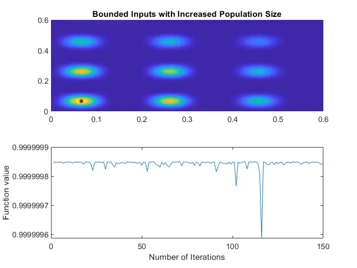
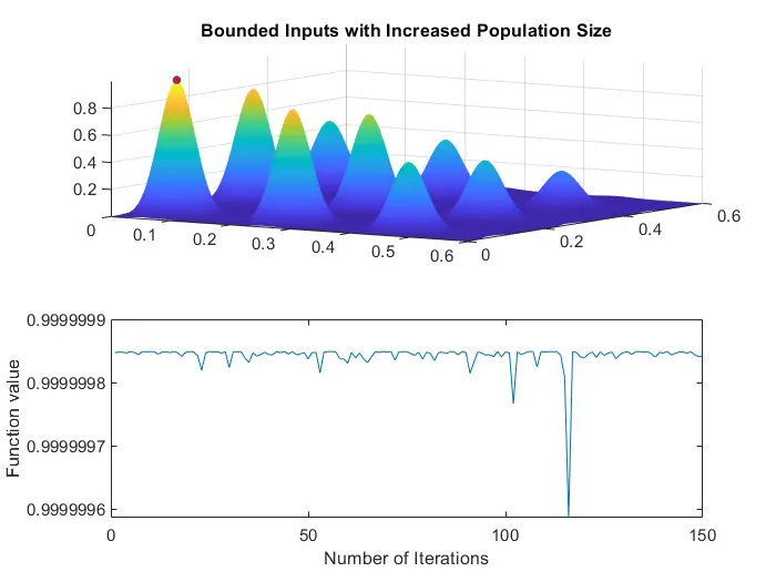
The value of global maxima can be observed as 0.99999985

Errors & steps taken to overcome

There was an error in reading the values for xx, yy in to the stalagmite function as the function was poorly defined. Later the error was overcome by reiterating the function code.
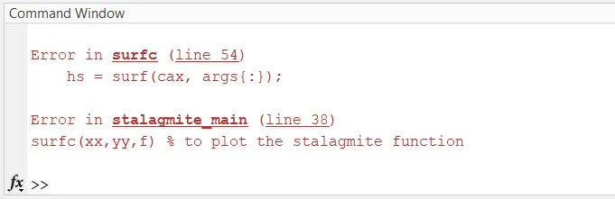
The below attached image is a reference to the error recieved in plotting the stalagmite function for the case studies. This was over come by correcting the argument.

References

Week 4.1 - Genetic Algorithm

Ship work like this
in your own course.

Talk to a career counsellor

Ship work like thisin your own course.

Talk to a career counsellor

Ship work like this
in your own course.