Project 2 - Rankine cycle Simulator
PROJECT 1 - RANKINE CYCLE SIMULATOR
AIM
To write a code in MATLAB to simulate the Rankine Cycle
Objective
- To create a Rankine Cycle Simulator using OCTAVE/MATLAB.
- To calculate the state points of the Rankine Cycle based on the inputs.
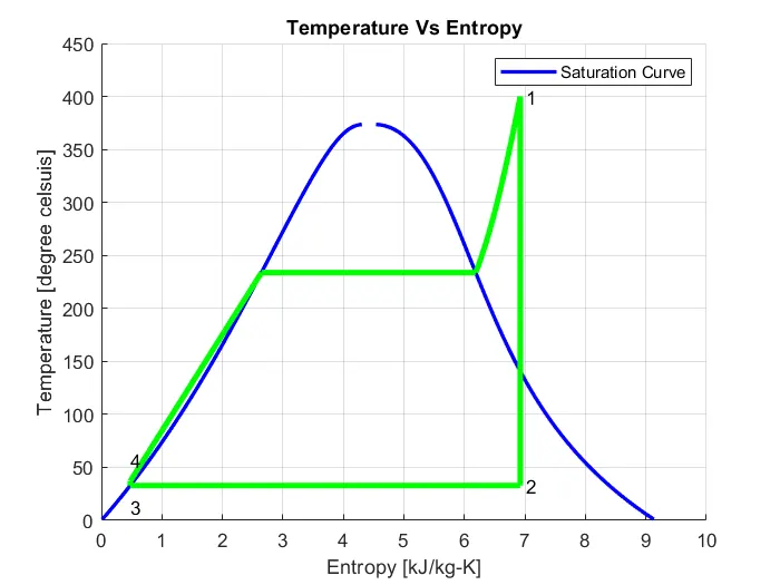
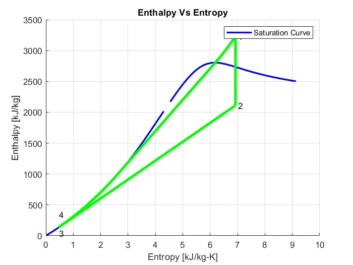
- Plot the corresponding T-s and h-s plots for the given set of inputs.
RANKINE CYCLE
The Rankine cycle is the fundamental operating cycle of all power plants where an operating fluid is continuously evaporated and condensed. The selection of operating fluid depends mainly on the available temperature range.
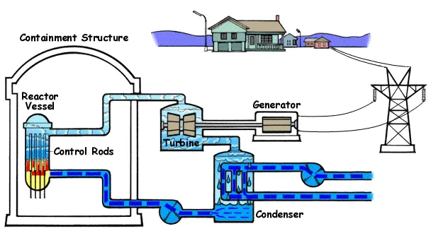
Rankine cycle consists pump, turbine, condenser, and boiler . Figure 1 shows the idealized Rankine cycle.
The pressure-enthalpy (p-h) and temperature-entropy (T-s) diagrams of this cycle are given in Figure 2. The Rankine cycle operates in the following steps:
-
1-2-3 Isobaric Heat Transfer. High pressure liquid enters the boiler from the feed pump (1) and is heated to the saturation temperature (2). Further addition of energy causes evaporation of the liquid until it is fully converted to saturated steam (3).
-
3-4 Isentropic Expansion. The vapor is expanded in the turbine, thus producing work which may be converted to electricity. In practice, the expansion is limited by the temperature of the cooling medium and by the erosion of the turbine blades by liquid entrainment in the vapor stream as the process moves further into the two-phase region. Exit vapor qualities should be greater than 90%.
-
4-5 Isobaric Heat Rejection. The vapor-liquid mixture leaving the turbine (4) is condensed at low pressure, usually in a surface condenser using cooling water. In well designed and maintained condensers, the pressure of the vapor is well below atmospheric pressure, approaching the saturation pressure of the operating fluid at the cooling water temperature.
-
5-1 Isentropic Compression. The pressure of the condensate is raised in the feed pump. Because of the low specific volume of liquids, the pump work is relatively small and often neglected in thermodynamic calculations.
Figure 1. Rankine cycle.
Figure 2. T-s and p-h diagrams.
The efficiency of power cycles is defined as
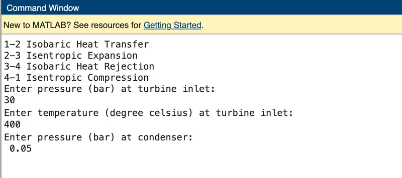
Required Inputs:
Turbine Inlet temperature = 400° C
Turbine Inlet Pressure = 30 bars
Turbine Outlet Pressure = 0.05 bars = Condenser Inlet Pressure
- Initially the part required to scan the inputs is compiled using input command and are assigned to the corresponding variables i.e. inlet pressure for turbine, temperature at turbine inlet and pressure at condenser.
- XSteam function file is used to read state point and the value of enthalpy and entropy at state point 1 is obtained.
- Since, 1-2 is isentropic compression the entropy at point 1 is equal to point 2. The term ‘(s_pT, p1, T1)’ refers to entropy at pressure and temperature point 1.
- The term ‘sg’ and ‘sf’ are referred to saturated liquid and saturated vapor entropy respectively. This value is used to calculate other function using mathematical relations.
- Similarly, parameters are calculated using other points which are taken from XSteam function file.
- Workdone in turbine and pump are calculated.
- The the net work done, the heat iput and output, the efficiency of the Rankine cycle are calculated along with specific steam consumption.
- Then temperature at each point of cycle is calculated using input taken from start of the program and data taken from XSteam file. For given temperature range from lower to higher, entropy points are calculated to create the T-S plot. Similarly, another for loop is used to create the saturation curve in each plot.
- Then, plotting is done respectively for T-s and H-s diagram and each state point value is displayed in command window.
PRIMARY CODE
%% RANKINE CYCLE SIMULATOR

close all
clear all
clc

% Description for print
fprintf('1-2 Isobaric Heat Transfer\n')
fprintf('2-3 Isentropic Expansion\n')
fprintf('3-4 Isobaric Heat Rejection\n')
fprintf('4-1 Isentropic Compression\n')

% Recieving Inputs
p1 = input('Enter pressure (bar) at turbine inlet:');
T1 = input('Enter temperature (degree celsius) at turbine inlet:');
p2 = input('Enter pressure (bar) at condenser:');

% Calculation of state points

% Point 1
h1 = XSteam('h_pt',p1,T1);
s1 = XSteam('s_pt',p1,T1);

% Point 2
s2=s1;
sf2 = XSteam('sL_p',p2);
sg2 = XSteam('sV_p',p2);
hf2 = XSteam('hL_p',p2);
hg2 = XSteam('hV_p',p2);
x2 = (s2-sf2)/(sg2-sf2);
h2 = hf2 + (x2*(hg2-hf2));
T2 = XSteam('T_hs',h2,s2);

% Point 3
T3 = T2;
p3 = p2;
s3 = XSteam('sL_T',T3);
h3 = XSteam('hL_T',T3);
v3 = XSteam('vL_p',p3);

% Point 4
p4 = p1;
s4 = s3;
Cp4 = XSteam('Cp_ps',p4,s4);
Cv4 = XSteam('Cv_ps',p4,s4);
% gamma = k
k = Cp4/Cv4;
r = (k-1)/k;
T4 = T3*(p4/p3)^r;

% Calculation of Output values

% Workdone by Turbine
Wt = h1-h2;

% Pump work
Wp = v3*(p1-p2)*100;
h4 = Wp + h3;
% Net workdone
Wnet = Wt - Wp;

% Heat
Qs = h1 - h4;
Qout = h2 - h3;

% Specific steam consumption
steam_rate = 3600/Wnet;

% Efficiency
n = (Wnet/Qs)*100;


% Saturated points
T6 = XSteam('Tsat_p',p1);
s5 = XSteam('sL_p',p1);
s6 = XSteam('sV_p',p1);
h5 = XSteam('hL_p',p1);
h6 = XSteam('hV_p',p1);
T5 = T6;

% Plotting Saturation curve
T = linspace(1,560,1000)
for i=1:length(T)
    sf(i)= XSteam('sL_T',T(i));
    sg(i)= XSteam('sV_T',T(i));
    hf(i)= XSteam('hL_T',T(i));
    hg(i)= XSteam('hV_T',T(i));
end


% Plotting T-S Diagram
figure(1)
hold on
plot(sf,T,'color','b','linewidth',2)
plot(sg,T,'color','b','linewidth',2)
plot([s1 s2],[T1 T2], 'color','g','linewidth',3)
plot([s2 s3],[T2 T3], 'color','g','linewidth',3)
plot([s3 s4],[T3 T4], 'color','g','linewidth',3)
plot([s4 s5],[T4 T5], 'color','g','linewidth',3)
plot([s5 s6],[T5 T6], 'color','g','linewidth',3)
S = linspace(s6,s1,1000)
for j=1:length(S)
    Tc(j) = XSteam('T_ps',p1,S(j));
end
plot(S,Tc,'color','g','linewidth',3)
text(s1+.1,T1,'1')
text(s2+.1,T2,'2')
text(s3,T3-20,'3')
text(s4,T4+20,'4')
title('Temperature Vs Entropy')
xlabel('Entropy [kJ/kg-K]')
ylabel('Temperature [degree celsuis]')
legend('Saturation Curve')
grid on


% Plotting H-S Diagram
figure(2)
hold on
plot(sf,hf,'color','b','linewidth',2)
plot(sg,hg,'color','b','linewidth',2)
plot([s1 s2],[h1 h2],'color','g','linewidth',3)
plot([s2 s3],[h2 h3],'color','g','linewidth',3)
plot([s3 s4],[h3 h4],'color','g','linewidth',3)
hc = linspace(h4,h5,1000)
for l=1:length(hc)
    sc(l) = XSteam('s_ph',p1,hc(l))
end
plot(sc,hc,'color','g','linewidth',3)
plot([s5 s6],[h5 h6],'color','g','linewidth',3)
for m=1:length(S)
    h_c(m)= XSteam('h_ps',p1,S(m));
end
plot(S,h_c,'color','g','linewidth',3)
text(s1+.1,h1,'1')
text(s2+.1,h2,'2')
text(s3,h3-100,'3')
text(s4,h4+200,'4')
title('Enthalpy Vs Entropy')
xlabel('Entropy [kJ/kg-K]')
ylabel('Enthalpy [kJ/kg]')
legend('Saturation Curve')
grid on


% Printing State Point Values
fprintf('Output\n')
fprintf('State point 1\nPressure (P1) : %10f bar\nTemperature (T1) : %11f degree celsius\nEnthalpy (H1) : %12f kJ/kg\nEntropy (S1) : %9f kJ/kgK\n\n',p1,T1,h1,s1)
fprintf('State point 2\nPressure (P2) : %10f bar\nTemperature (T2) : %11f degree celsius\nEnthalpy (H2) : %12f kJ/kg\nEntropy (S2) : %9f kJ/kgK\n\n',p2,T2,h2,s2)
fprintf('State point 3\nPressure (P3) : %10f bar\nTemperature (T3) : %11f degree celsius\nEnthalpy (H3) : %12f kJ/kg\nEntropy (S3) : %9f kJ/kgK\n\n',p3,T3,h3,s3)
fprintf('State point 4\nPressure (P4) : %10f bar\nTemperature (T4) : %11f degree celsius\nEnthalpy (H4) : %12f kJ/kg\nEntropy (S4) : %9f kJ/kgK\n\n',p4,T4,h4,s4)
fprintf('Turbine Workdone(Wt) : %14f kJ/kg\nPump Workdone(Wp) : %14f kJ/kg\nNet Workdone(Wnet) : %14f kJ/kg\nThermal Efficiency(n) : %4.2f percent\nSpecific Steam Consumption : %f kg/kJ',Wt,Wp,Wnet,n,steam_rate)
OUTPUT
T-S Diagram
H-S diagram
The output window for scanning of INPUTS is shown below:
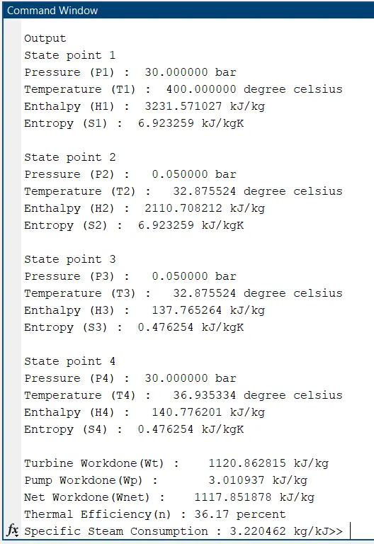
The output for the calculation of STATE POINTS for the inputs defined in the challenge is shown below:
Errors Faced and steps taken to overcome
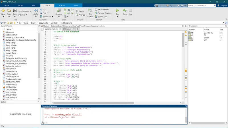
- While evaluating the program for the first time, the error mentioned in the below image was shown. It was identified as unrecognized function 's1' in line21. The error was cleared by defining p1 instead of s1.
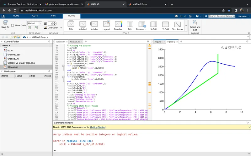
- The following error was thrown while running the program as 'array indices must be positive integers or logical values'. The error was identified in line106 in plotting the H-S diagram and was cleared by defining the proper variable inside the for loop. ('l' instead of 'k')
REFERNCES
https://in.mathworks.com/help/
https://thermopedia.com/content/1072
https://www.researchgate.net/publication/328576312_rankine_cycle
https://www.wikipedia.org/