Week 3 - Solving second order ODEs

Aim

To write a program in matlab to simulate an ODE representing the Simple Harmonic Motion of a pendulum and to animate the motion of the pendulum for the given parameters.

Second Order Differential Equation

A second order differential equation is defined as a differential equation that includes a function and its second-order derivative and no other higher-order derivative of the function can appear in the equation. It can be of different types depending upon the power of the derivative and the functions involved. These differential equations can be solved using the auxiliary equation. An example for Second order derivative is pendulum motion.

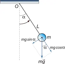
In order to solve 2nd order ODE's, it is simplified in to smaller order derivatives using auxiliary equations. The second order derivative for the motion of a pendulum is given as:

In the above equation,

g = gravity in m/s2,

L = length of the pendulum in m,

m = mass of the ball in kg,

b=damping coefficient.

Simplifying the above equation:

theta = theta1

Therefore dtheta/dt = dtheta1/dt

dtheta1/dt = theta2 ----------- (1).

d^2theta/dt^2 ---> d^2theta1/dt^2

d/dt(dtheta1/dt) = dtheta2/dt --------(2).

In order to simulate the motion of the pendulum, functions are used to compile the second order derivative equation and later the function is called in the main function. Equations (1) and (2) are implied to theta(1) and theta(2) in compiling inside the function.

Function code to solve equation

function[dtheta_dt]= pendulum_func(t,theta,b,g,l,m)

theta1 = theta(1)
theta2 = theta(2)
dtheta1_dt = theta2;
dtheta2_dt = -(b/m)*theta2 - (g/l)*sin(theta1);

dtheta_dt = [dtheta1_dt; dtheta2_dt];
end

Code to simulate pendulum motion

The input parameters are taken and the function pendulum_func is called in receiving the input values. The inbuilt solver ode45 {format:[t,y] = ode45(odefun,tspan,y0)} is used to solve the second order derivative.

%% Solving second order ODE (Simple pendulum oscillation)

clear all
close all 
clc

% Input variables
b = .05;
g = 9.81;
m = .1;
l = 1;

% Initial conditions
% giving initial velocity and the angle
theta_0 = [0;3];

% Time pionts
t_span = linspace(0,20,500);

% Solving ODE
[t,results] = ode45(@(t,theta) pendulum_func(t,theta,b,g,l,m),t_span,theta_0);


% To defined pivot point of pendulum and plot it.
x0=0;
y0=0;
plot(x0, y0,'marker', 'o')

% To extract the first column of a result and assigned it to 'y'
y =  results(:,1);  % Theta/Angular displacement

figure(1)
plot(t,results(:,1))
hold on
plot(t,results(:,2)) 
grid on
xlabel('Time')
ylabel('Plot')
legend('Angular Displacement','Angular Velocity','location','southeast')
title('Time vs Plot') 

% To create images for each time value and stored it in array ‘M’.
ct=1;
for i=1:length(t_span)   % i=1,2,3,4,5,,,,,,20
    x1 = l*sin(y(i));
    y1= -l*cos(y(i));
    figure(2)
    plot([x0 x1],[y0 y1],'linewidth',3,'marker','o')
    hold on
    plot(x1, y1, 'marker','o', 'color','g','markersize',30, 'markerfacecolor', 'g')
    hold off 
    title({'Simple harmonic motion'; 'of a pendulum'}, 'color','r')
    axis([-1 1 -2 0])
    pause(0.01)
    M(ct)= getframe(gcf);
    ct=ct+1;
end

%  To create animation of S.H.M. of simple pendulum
movie(M)
videofile = VideoWriter('pendulum.avi', 'Uncompressed AVI');
open(videofile)
writeVideo(videofile,M)
close(videofile)

Output plot for Angular Velocity and Angular Displacement to Time

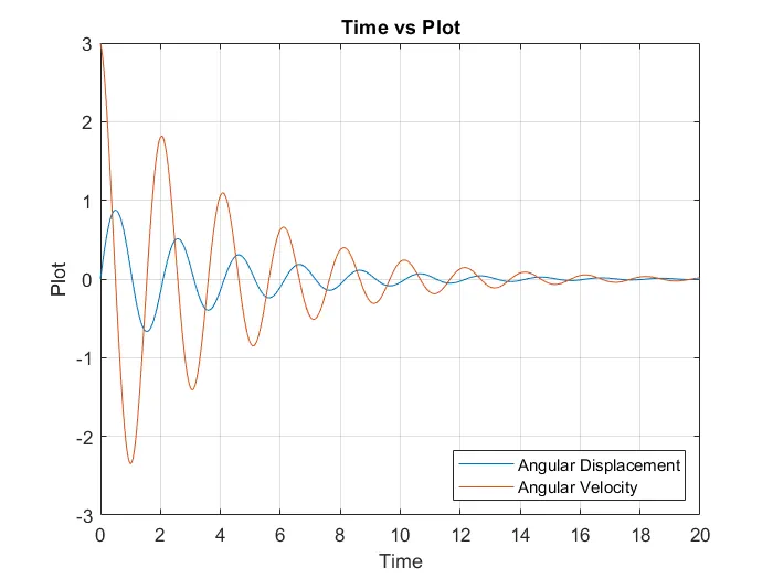
The animation is then compiled by stitching individual frames captured in the variable using various video writing commands.

Output - Video file link

https://youtu.be/ojxjJAG0BPw

References

Previous student projects.

https://www.cuemath.com/calculus/second-order-differential-equation/

https://www.google.com/