MATLAB Scripting of 4th Order Central & Upwind Scheme using Taylor table method

Objective

Deriving the 4th order approximations of the second-order derivative for Central difference, Skewed right-sided difference & Skewed left-sided difference Scheme.

Writing a MATLAB Code to evaluate the second-order derivative of the analytical function exp(x)*cos(x) and compare it with the 3 derived numerical approximations.

Creating a plot that compares the absolute error between the above-mentioned schemes.

Solution

Taylor's Table method is used to Derive the 4th order approximations of the second-order derivative for Central difference, Skewed right-sided difference & Skewed left-sided difference Scheme.

Skewed right-sided difference Scheme

The number of nodes in the stencil N for a given accuracy we can calculate using this formula.

Number of nodes in the stencil N = The order of accuracy P + order of derivative Q

P = 4 (We need 4th order accurate scheme)

Q = 2 (Second Order Derivative)

So we need to consider N = 6 nodes in our stencil.

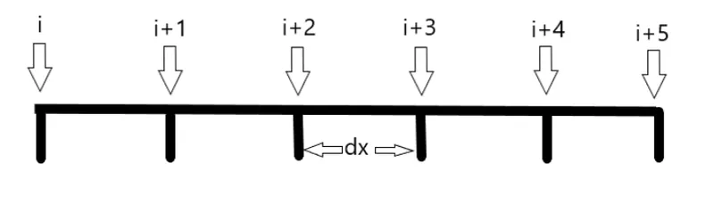
So we can write a general Skewed right-sided 4th Order difference Scheme formula as:-

`(deltax)^2*(d^2f)/(dx^2) = a*f_i + b*f_(i+1) +c*f_(i+2) + d*f_(i+3) + e*f_(i+4) + g*f_(i+5)`

a,b,c,d,e,g coefficients can be calculated via Taylor's Table Method

	`f(i)`	`deltaxf'(i)`	`deltax^2f''(x)`	`deltax^3f'''(x)`	`deltax^4f^(iv)(x)`	`deltax^5f^v(x)`
`a*f_i`	a	0	0	0	0	0
`b*f_(i+1)`	b	b	b/2	b/6	b/24	b/120
`c*f_(i+2)`	c	2c	4c/2	8c/6	16c/24	32c/120
`d*f_(i+3)`	d	3d	9d/2	27d/6	81d/24	243d/120
`e*f_(i+4)`	e	4e	16e/2	64e/6	256e/24	1024e/120
`g*f_(i+5)`	g	5g	25g/2	125g/6	625g/24	3125g/120
`deltax^2f''(x)`	0	0	1	0	0	0

So we have 6 algebric equations

`a+b+c+d+e+g=0`

`b+2c+3d+4e+5g=0`

`b/2+(4c)/2+(9d)/2+(16e)/2+(25g)/2=1`

`b/6+(8c)/6+(27d)/6+(64e)/6+(125g)/6=0`

`b/24+(16c)/24+(81d)/24+(256e)/24+(625g)/24=0`

`b/120+(32c)/120+(243d)/120+(1024e)/120+(3125g)/120=0`

After solving these 6 equation, The 4th order right side skewed scheme is as follow:-

`(d^2f)/(dx^2) = ((15/4)*f_i + (-77/6)*f_(i+1) +(107/6)*f_(i+2) - 13*f_(i+3) + (61/12)*f_(i+4) + (-5/6)*f_(i+5))/(deltax)^2`

Skewed left-sided difference Scheme

The number of nodes in the stencil N for a given accuracy can be calculated using the same formula

Number of nodes in the stencil N = The order of accuracy P + order of derivative Q

P = 4 (We need 4th order accurate scheme)

Q = 2 (Second Order Derivative)

So we need to consider N = 6 nodes in our stencil.

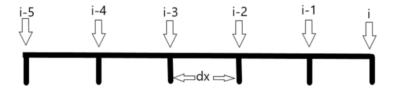
So we can write a general Skewed left-sided 4th Order difference Scheme formula as:-

`(deltax)^2*(d^2f)/(dx^2) = a*f_i + b*f_(i-1) +c*f_(i-2) + d*f_(i-3) + e*f_(i-4) + g*f_(i-5)`

a,b,c,d,e,g coefficients can be calculated via Taylor's Table Method

	`f(i)`	`deltaxf'(i)`	`deltax^2f''(x)`	`deltax^3f'''(x)`	`deltax^4f^(iv)(x)`	`deltax^5f^v(x)`
`a*f_i`	a	0	0	0	0	0
`b*f_(i-1)`	b	-b	b/2	-b/6	b/24	-b/120
`c*f_(i-2)`	c	-2c	4c/2	-8c/6	16c/24	-32c/120
`d*f_(i-3)`	d	-3d	9d/2	-27d/6	81d/24	-243d/120
`e*f_(i-4)`	e	-4e	16e/2	-64e/6	256e/24	-1024e/120
`g*f_(i-5)`	g	-5g	25g/2	-125g/6	625g/24	-3125g/120
`deltax^2f''(x)`	0	0	1	0	0	0

So we have 6 algebric equations

`a+b+c+d+e+g=0`

`-b-2c-3d-4e-5g=0`

`b/2+(4c)/2+(9d)/2+(16e)/2+(25g)/2=1`

`-b/6-(8c)/6-(27d)/6-(64e)/6-(125g)/6=0`

`b/24+(16c)/24+(81d)/24+(256e)/24+(625g)/24=0`

`-b/120-(32c)/120-(243d)/120-(1024e)/120-(3125g)/120=0`

After solving these 6 equation, The 4th order left side skewed scheme is as follow:-

`(d^2f)/(dx^2) = ((15/4)*f_i + (-77/6)*f_(i-1) +(107/6)*f_(i-2) - 13*f_(i-3) + (61/12)*f_(i-4) + (-5/6)*f_(i-5))/(deltax)^2`

Central difference Scheme

The formula to calculate the number of nodes in the stencil N for the central difference is slightly different and shown below.

Number of nodes in the stencil N = The order of accuracy P + order of derivative Q - 1

So we need to consider N = 5 nodes in our stencil.

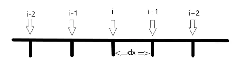
So we can write a general Central 4th Order difference Scheme formula as:-

`(deltax)^2*(d^2f)/(dx^2) = a*f_(i-2) + b*f_(i-1) + c*f_(i)+ d*f_(i+1) + e*f_(i+2)`

a,b,c,d,e coefficients can be calculated via Taylor's Table Method

	`f(i)`	`delta(x)*f'(i)`	`deltax^2*f''(i)`	`deltax^3*f'''(i)`	`deltax^4*f^(iv)(i)`
`a*f_(i-2)`	a	-2a	4a/2	-8a/6	16a/24
`b*f_(i-1)`	b	-b	b/2	-b/6	b/24
`c*f_(i)`	c	0	0	0	0
`d*f_(i+1)`	d	d	d/2	d/6	d/24
`e*f_(i+2)`	e	2e	4e/2	8e/2	16e/24
`deltax^2*f''(x)`	0	0	1	0	0

So we have 5 algebric equations

`a+b+c+d+e=0`

`-2a-b+d+2e=0`

`(4a)/2+b/2+d/2+(4e)/2=1`

`-(8a)/6-b/6+d/6+(8e)/6=0`

`(16a)/24+b/24+d/24+(16e)/24=0`

After solving these 5 equation, The 4th order central difference scheme is as follow:-

`(d^2f)/(dx^2) = ((-1/12)*f_(i-2) + (4/3)*f_(i-1) + (-5/2)*f_(i)+ (4/3)*f_(i+1) + (-1/12)*f_(i+2))/(delta(x)^2)`

MATLAB Code to evaluate the second-order derivative and compare it with the 3 derived numerical approximations

Analytical Function = `e^(x)*cos(x)`

x = `pi/3`

x range = pi/4000 to pi/4 with 20 intervals

so dx will be an array starting from pi/4000(smallest size) to pi/4(largest size).

Code Logic

Separate codes are written for all three schemes where all algebraic equations(obtained from Taylor's Method) are stored and coefficients for the numerical schemes are calculated using an inbuilt MATLAB solver. Then numerical derivative & numerical error is evaluated for all three schemes.

Numerical Error = |Analytical Derivative - Numerical Derivative|

The Main code will take user input of the value of approximation x which is assigned as pi/3.

Then the main code will take input for grid spacing.

max_dx = pi/4

min_dx = pi/4000

Number of interval = 20

Then using a for loop, all three separate codes are called, In which then numerical error for the complete grid is calculated and stored in a separate array.

Later log-log Plot instead of the standard plot is used to plot the error for all three schemes for the different sizes of dx values.

log-log plot helps us to compare the curves with different magnitude ranges on a log scale easily.

Code for 4th Order Central Difference Scheme

function error = central_difference_scheme(x,dx)

%analytical function = exp(X)*cos(X)
analytical_derivative = -2*exp(x)*sin(x);

f = @(x) exp(x)*cos(x);

%fourth order central difference formula
% f''(x) = a*f(i-2) + b*f(i-1) + c*f(i) + d*f(i+1) + e*f(i+2)
%calculating the arbitary constant (a,b,c,d,e)

syms a b c d e               %Creating symbolic variables

%system of equations obtained from taylor's table

eqn1 = a + b + c + d + e  == 0;
eqn2 = -2*a - b + d + 2*e == 0;
eqn3 = 2*a + b/2 + d/2 + 4*e/2 == 1;
eqn4 = -8*a/6 - b/6 + d/6 + 8*e/6 == 0;
eqn5 = 16*a/24 + b/24 + d/24 + 16*e/24 == 0;

equation = [eqn1 eqn2 eqn3 eqn4 eqn5];

solution = solve(equation);      %Solving a system of equations

%accessing the coefficients from the structure s
a = solution.a;
b = solution.b;
c = solution.c;
d = solution.d;
e = solution.e;

central_difference = (a*f(x-2*dx) + b*f(x-dx) + c*f(x) + d*f(x+dx) + e*f(x+2*dx))/(dx^2);

error = abs(central_difference - analytical_derivative);

end

Code for 4th Order Skewed left-sided difference Scheme

function error = left_side_skewed_scheme(x,dx)

%analytical function = exp(X)*cos(X)
analytical_derivative = -2*exp(x)*sin(x);

f = @(x) exp(x)*cos(x);

%fourth order left side skewed difference formula
% f''(x) = a*f(i) + b*f(i-1) + c*f(i-2) + d*f(i-3) + e*f(i-4) + g*f(i-5)
%calculating the arbitary constant (a,b,c,d,e,,g)

syms a b c d e g               %Creating symbolic variables

%system of equations obtained from taylor's table

eqn1 = a + b + c + d + e + g  == 0;
eqn2 = -b - 2*c - 3*d - 4*e - 5*g == 0;
eqn3 = b/2 + 4*c/2 + 9*d/2 + 16*e/2 + 25*g/2 == 1;
eqn4 = -b/6 - 8*c/6 - 27*d/6 - 64*e/6 - 125*g/6 == 0;
eqn5 = b/24 + 16*c/24 + 81*d/24 + 256*e/24 + 625*g/24 == 0;
eqn6 = -b/120 -32*c/120 -243*d/120 - 1024*e/120 - 3125*g/120 == 0;

equation = [eqn1 eqn2 eqn3 eqn4 eqn5 eqn6];

solution = solve(equation);      %Solving a system of equations

%accessing the coefficients from the structure s
a = solution.a;
b = solution.b;
c = solution.c;
d = solution.d;
e = solution.e;
g = solution.g;

left_skew_difference = (a*f(x) + b*f(x-dx) + c*f(x-2*dx) + d*f(x-3*dx) + e*f(x-4*dx) + g*f(x-5*dx))/(dx^2);

error = abs(left_skew_difference - analytical_derivative);

end

Code for 4th Order Skewed right-sided difference Scheme

function error = right_side_skewed_scheme(x,dx)

%analytical function = exp(X)*cos(X)
analytical_derivative = -2*exp(x)*sin(x);

f = @(x) exp(x)*cos(x);

%fourth order right side skewed difference formula
% f''(x) = a*f(i) + b*f(i+1) + c*f(i+2) + d*f(i+3) + e*f(i+4) + g*f(i+5)
%calculating the arbitary constant (a,b,c,d,e,g)

syms a b c d e g               %Creating symbolic variables

%system of equations obtained from taylor's table

eqn1 = a + b + c + d + e + g  == 0;
eqn2 = b + 2*c + 3*d + 4*e + 5*g == 0;
eqn3 = b/2 + 4*c/2 + 9*d/2 + 16*e/2 + 25*g/2 == 1;
eqn4 = b/6 + 8*c/6 + 27*d/6 + 64*e/6 + 125*g/6 == 0;
eqn5 = b/24 + 16*c/24 + 81*d/24 + 256*e/24 + 625*g/24 == 0;
eqn6 = b/120 + 32*c/120 + 243*d/120 + 1024*e/120 + 3125*g/120 == 0;

equation = [eqn1 eqn2 eqn3 eqn4 eqn5 eqn6];

solution = solve(equation);      %Solving a system of equations

%accessing the coefficients from the structure s
a = solution.a;
b = solution.b;
c = solution.c;
d = solution.d;
e = solution.e;
g = solution.g;

right_skew_difference = (a*f(x) + b*f(x+dx) + c*f(x+2*dx) + d*f(x+3*dx) + e*f(x+4*dx) + g*f(x+5*dx))/(dx^2);

error = abs(right_skew_difference - analytical_derivative);

end

Main Code

clc
clear all
close all

disp('Analytical Function is exp(x)*cos(x)')

%taking the input for x

x = input('Enter the value of approximation ');

%taking the input for grid spacing
max_dx = input('Enter the value of max step size');
min_dx = input('Enter the value of min step size');
num    = input('Enter the nuumber of interval');

dx = linspace(max_dx,min_dx,num);

for i = 1:length(dx)
    central_diff_error(i) = central_difference_scheme(x,dx(i));
    left_skewed_error(i)  = left_side_skewed_scheme(x,dx(i));
    right_skewed_error(i) = right_side_skewed_scheme(x,dx(i));
end

figure(1)
loglog(dx,central_diff_error,'LineWidth',2)
hold on

loglog(dx,left_skewed_error,'r','LineWidth',2)
loglog(dx,right_skewed_error,'g','LineWidth',2)

xlabel('Mesh Size','fontsize',12,'fontweight','bold')
ylabel('Numerical Error','fontsize',12,'fontweight','bold')

legend('Central 4th Order Difference','Left Side Skewed 4th Order Difference','Right Side Skewed 4th Order Difference','FontSize',14)
legend('Location','northwest')

text(0.001,1,'f(x) = exp(x)*cos(x)','FontSize', 13)

Results & Discussions

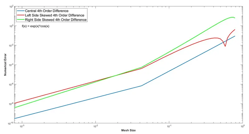
Error for Central Difference Scheme is leaste.

Error for Right Sied Skewed and Left Side Skewed Scheme is quite similar.

For the coarse grid spacing ~ 0.1, Left Side Skewed Scheme gives less error.

For the fine grid spacing ~ 0.001, Right Side Skewed Scheme gives less error.

Skewed Scheme is useful for convection dominating flow, In these type of flow Skewed schemes are highly stable where as Central Difference scheme is unstable This is because for convection dominating flow, Value at current node will be only affected or influenced by upstream side nodes.

So if we take the information from both sides as we do it in Central Difference Scheme, It will make the solution unstable.

High Order Central Difference Scheme can't be used near or to boundary node because of unavailability of boudnary side nodes.