Solving second order ODEs using MATLAB (Motion of a simple pendulum with damping)

Objective

Solve the motion of Simple Pendulum with damping using a second-order ODE.

`(d^2theta)/dt^2 + b/m(d(theta))/dt +g/L(Sintheta) = 0`

In this equation, Theta is the angular displacement of the pendulum. Solve the equation to get angular displacement and velocity of a pendulum with respect to time.

Plot displacement and velocity of a pendulum with respect to time and how is the damping nature of the system.

Create an animation of the pendulum motion with respect to time.

Introduction

This is the second order Ordinary Differential Equation. This equation describes a lot of engineering applications for example motion of a simple pendulum, motion of a spring-mass, and a damper system. By giving an initial condition we can solve the above ODE and analyze how the mass moves with respect to time. The solution of that ODE can give useful information about the system such that displacement and velocity of the pendulum.

Input

L=1 metre (Length of pendulum)

m=1 kg (Mass of pendulum)

b=0.05 (damping coefficient)

g=9.81 m/s2 (acceleration due to gravity)

Initial Condition

Initial Displacement is 0

Initial Velocity is 3 radian/s.

Solution

I have written a code by defining the input, initial condition in an array, time limits for integrating the ODE then I have used the ODE45 solver available in MATLAB to solve the ODE.

I have rewritten the second-order ODE into two first-order ODEs as follow:-

`(d^2theta)/dt^2 + b/m(d(theta))/dt +g/L(Sintheta) = 0`

`theta` is displacement.

Let's define

`theta = theta_1`

`(d(theta_1))/dt = theta_2`

where as `theta2` is angular velocity.

Now we can write our 2 First-order ODEs as follow:-

`(d(theta_1))/dt = theta_2`

Solution of the above equation will give the angular displacement.

`(d(theta_2))/dt + (b/m)theta_2 +(g/L)sin(theta_1) = 0`

Solution of the above equation will give the angular velocity.

Both ODEs are of the order first.

Now both ODEs can be scripted into the MATLAB using ode45 solver to solve the motion of Simple Pendulum as shown below.

MATLAB CODE

%SOLVING PENDULUM MOTION USING A SECOND ORDER ODE

clc
clear all
close all

b = 0.05;  %damping coeff
m = 0.1;  %mass of the pendulum
g = 9.81; %acceleration due to gravity
l = 1;  %length of pendulum in meters

%innitial_condition 

theta_0 = [0;3]; %innitial displacement is 0 and innitial velocity is 3 radian/s

%integrating the ODE system to obtain a solution

t_span = linspace(0,20,400); %time goes from 0 to 20 seconds with 1000 steps

%solve ODE using ODE Function

%ODE is a function of time and angle 
%parameters ode_func is used to define our input and called from a function
% then we proive out innitial condition and time lower &  upper limit

[t, results] = ode45(@(t,theta) ode_func(t, theta, b, m, l ,g), t_span, theta_0);

%plotting

plot(t,results(:,1)); %plotting time vs displacement
hold on;
plot(t,results(:,2)); %plotting time vs velocity
ylabel('Plot');
xlabel('Time');

pause(3)
close all

%animating the pendulum as a function of time

time = t;   %storing the time array

displacement = results(:,1); %storing the displacement array

ct = 1;

for i = 1:length(time)
    
    %current coordiantes of pendulme 
    x1 =  sin(displacement(i));
    y1 = -cos(displacement(i));
    
    %coordinate at where pendulum is fixed
    x0 = 0;             
    y0 = 0;                   
    
    plot(x1,y1,'ko',[-1 1 x0 x1],[0 0 y0 y1],'k-','MarkerFaceColor','k','linewidth',3)
    axis([-1.2 1.2 -1.2 0.2])            %set x and y axis limit
    pause(0.3) 
    M(ct) = getframe(gcf)             %capturing the current frame figure
    ct = ct+1;                        %incrementing the frame
end

movie(M)                                  %generate movie with all frame
videofile = VideoWriter('pendulum_animation.avi','Uncompressed AVI')     %create new video file to store all frames
open(videofile)                                       %open up the file
writeVideo(videofile,M)                               %write all frames of video
close(videofile)                                      %close the file

Explanation of the key logic used in the above code.

In the above code, A separate function to break our second order ODE into two first-order ODE using "ode_func"

In ode_func, we are calling the input parameters such as damping coefficient, length & mass of the pendulum, and then formulating the two first-order ODEs.

The output of "ode_func" gives a column vector where the output of 2 first-order ODEs are stored which is angular displacement and angular velocity.

Later this "ode_func" is called in the main code by the ODE45 solver to get the displacement and velocity with respect to time.

For the animation part, A For loop is used in Time that captures the displacement x and y coordination location of the pendulum as it moves with time.

A plot is created for the movement of the pendulum.

getframe command is used to capture all the motion frame of a pendulum within the time loop.

All frames are stored in memory and then used to create a Movie using movie command.

MATLAB Code for ode_func

%defining our input for pendulum simulation 

function [dtheta_dt] = ode_func(t, theta, b, m, l ,g)

    %theta is our solution array
    theta1 = theta(1);   %angualr displacement
    theta2 = theta(2);   %angular velocity
    dtheta1_dt = theta2; %taking time derivative of theta1, our first ode
    dtheta2_dt = -(b/m)*theta2 - (g/l)*sin(theta1); %taking time derivative of theta2, our second ode
    dtheta_dt = [dtheta1_dt;dtheta2_dt];
end

Results

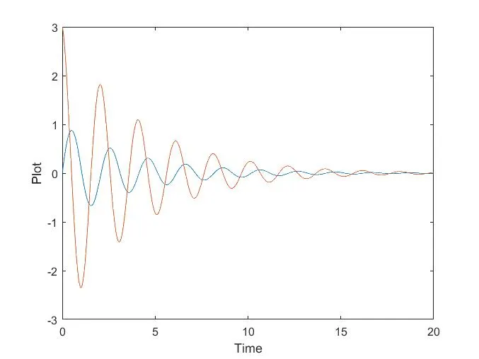
We can see pendulum starts from an Initial Displacement of 0 and Initial Velocity is 3 radian/s and as time goes on, the Motion of the pendulum relaxes and comes to a rest.

Animated Video Link:-

https://drive.google.com/file/d/1tsupIoBcAE00rc9jfhAa0ptmxQ8ms5-D/view?usp=sharing

Animation of the motion of the pendulum can be found in the above link which is governed by Second-Order ODE. In the video, we can clearly see the Motion of the pendulum relax and comes to a rest.