Optimization of Stalagmite Function using Genetic Algorithm in MATLAB

Objective

Write a code in MATLAB to optimize the stalagmite function and find the global maxima of the function.

Explain the concept of genetic algorithm and the syntax for ga in MATLAB.

Plot the stalagmite function and the function maximum value for a given search space using GA solver under 3 conditions - Unbounded Input, Bounded Input and Increased Population Size.

Theory for Genetic Algorithm

A genetic algorithm is a search heuristic that is inspired by Charles Darwin’s theory of natural evolution. This algorithm reflects the process of natural selection where the fittest individuals are selected for reproduction in order to produce offspring of the next generation.

The process of natural selection starts with the selection of the fittest individuals from a population. They produce offspring which inherit the characteristics of the parents and will be added to the next generation. If parents have better fitness, their offspring will be better than parents and have a better chance of surviving. This process keeps on iterating and in the end, a generation with the fittest individuals will be found.

Five phases are considered in a genetic algorithm.

1. Initial population
2. Fitness function
3. Selection
4. Crossover
5. Mutation
6. Termination

Initial Population

The process begins with a set of individuals which is called a Population. Each individual is a solution to the problem you want to solve. An individual is characterized by a set of parameters (variables) known as Genes. Genes are joined into a string to form a Chromosome (solution).

Fitness Function

The fitness function determines how fit an individual is (the ability of an individual to compete with other individuals). It gives a fitness score to each individual. The probability that an individual will be selected for reproduction is based on its fitness score.

Selection

Two pairs of individuals (parents) are selected based on their fitness scores. Individuals with high fitness have more chances to be selected for reproduction.

Crossover

For each pair of parents to be mated, a crossover point is chosen at random from within the genes. Offspring are created by exchanging the genes of parents among themselves until the crossover point is reached. The new offspring are added to the population.

Mutation

In certain new offspring formed, some of their genes can be subjected to a mutation with a low random probability. The key idea is to insert random genes in offspring to maintain the diversity in the population to avoid premature convergence.

Termination

The algorithm terminates if the population has converged (does not produce offspring which are significantly different from the previous generation). Then it is said that the genetic algorithm has provided a set of solutions to our problem.

Syntax of Genetic Algorithm in MATLAB

x = ga(fun,nvars)

MATLAB Code for formulating stalagmite function

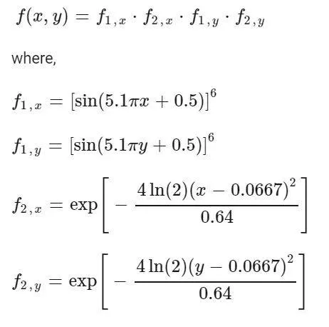
function [stag] = get_stalagmite(x,y)

[xx yy] = meshgrid(x,y);

for i = 1:length(xx)
    for j = 1:length(yy)       %generating data for the plot
        inputvector(1) = xx(i,j);   %storing x value of meshgrid in an array
        inputvector(2) = yy(i,j);   %storing y value of meshgrid in an array
    end
end

f_x_1 = (sin(5.1*xx*pi + 0.5)).^6;

f_y_1 = (sin(5.1*yy*pi + 0.5)).^6;

f_x_2 = exp(-4*log(2)*(((xx-0.0667).^2)/0.64));

f_y_2 = exp(-4*log(2)*(((yy-0.0667).^2)/0.64));

stag = -(f_x_1.*f_x_2.*f_y_1.*f_y_2);

end

function [stag] = stalagmite(inputvector)

x = inputvector(1);
y = inputvector(2);

f_x_1 = (sin(5.1*x*pi + 0.5)).^6;

f_y_1 = (sin(5.1*y*pi + 0.5)).^6;

f_x_2 = exp(-4*log(2)*(((x-0.0667).^2)/0.64));

f_y_2 = exp(-4*log(2)*(((y-0.0667).^2)/0.64));

stag = -(f_x_1*f_x_2*f_y_1*f_y_2);

end

Study-1

I have defined a search space in which x and y location varies from 0 to 0.6 In this search space. I have plotted the stalagmite function in this search space.

For the study-1, This search space is not directly assigned to the GA solver. Meaning the GA solver does not know that the optimum function value should not go beyond 0.6 and below 0.

clear all
close all
clc

%create 1d input array
%defining our search space

x = linspace(0,0.6,150);
y = linspace(0,0.6,150);
num_iteration = 50;       %running genetic algorithm 50 times
f = get_stalagmite(x,y);  %generates stalagmite function

%performing geneatic algorithm
%using ga we are minimizing the stalagmite function, 2- no. of variables
%inputs - getting the optimum minimum value

tic

%Study - 1 Statistical Behavior (Unbounded)

%calling the genetic algorithm solver 

for i = 1:num_iteration
    [inputs, fval(i)] = ga(@stalagmite, 2);
    xval(i) = inputs(1);
    yval(i) = inputs(2);
end

run_time_study_1 = toc

figure(1)             %open a new figure window
subplot(2,1,1)        %creating multiple plot in a single figure
hold on

surfc(x,y,f)          %surface plot to visualize the stalagmite function
shading interp        %to avoid contour lines in surface plot

%Plotting optimum value predicted by GA solver over the 50 studies

plot3(xval,yval,fval,'marker','o','markersize',5,'markerfacecolor','r') 
xlabel('X-Coordinate')
ylabel('Y-Coordinate')

title('Unbounded Inputs')
subplot(2,1,2)       %creating another subplot
plot(fval)           %ploting optimum value predicted by GA as a function of iteration
xlabel('Iterations')
ylabel('Solution Minimum')

Observation - Study 1 (Unbounded Results)

Run Time = 4.78 seconds

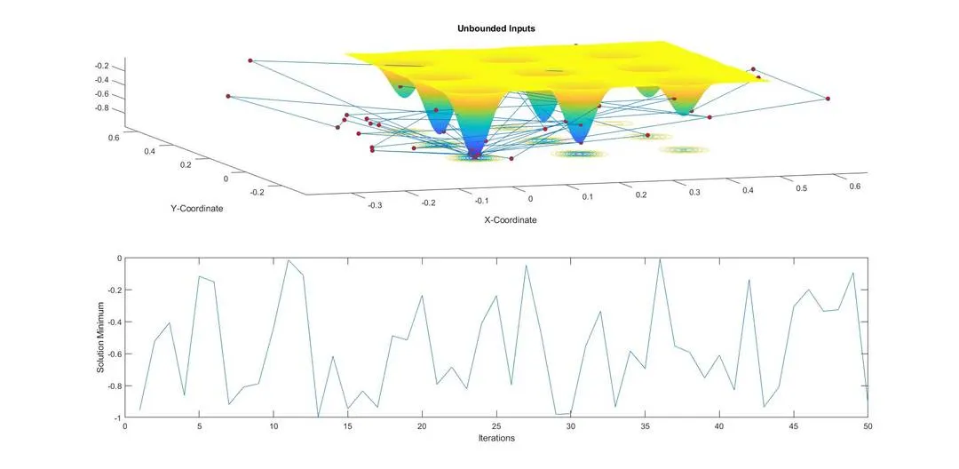
The upper 3d plot plots stalagmite function and the minimum value is also plotted which is predicted by GA solver. We can see it is scattered all over the place. It is unbounded as well because the value predicted is outside the search space for some iterations. This happens because of random sampling. We haven't told the GA solver explicitly that what is the search space where the GA solver should restrict the sampling.

In the bottom plot, I have plotted the optimum value predicted by the GA solver over the iterations. We can see for each iteration minimum value changes between 0 and -1.

Study-2 Code

Here we have set up the bounds for the variables x and y which will make sure that GA Solver doesn't go out of these bounds.

%Study - 2 Statistical Behavior (With Upper and Lower Bound)

%previously, our optimum value coordinatas was going beyond 0 and 0.6
%Here we will define the search space for GA Solver explicitly

tic

for i = 1:num_iteration
    [inputs, fval(i)] = ga(@stalagmite, 2, [], [], [], [], [0;0],[1;1]);  %giving x & y upper and lower limit
    xval(i) = inputs(1);
    yval(i) = inputs(2);
end

run_time_study_2 = toc

figure(2)             
subplot(2,1,1)        
hold on

surfc(x,y,f)          
shading interp        

plot3(xval,yval,fval,'marker','o','markersize',5,'markerfacecolor','r')
xlabel('X-Coordinate')
ylabel('Y-Coordinate')
title('Bounded Inputs')
subplot(2,1,2)       
plot(fval)           
xlabel('Iterations')
ylabel('Solution Minimum')

Observation - Study 2 (Bounded Results)

Run Time = 5.44 seconds

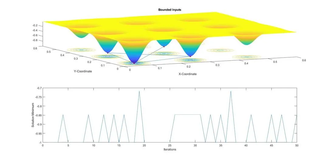
Now GA solver predicts value within the function range between the peaks which is much better than our previous case. It predicts those big 4 peaks as optimum value.

In the below graph we can see the minimum value is between -0.7 and -1 which is a much narrow range. Now to improve the accuracy we have to reduce the search space.

Study-3 Code

The genetic algorithm starts with a random sample. The default sample is 50. Here we have 2 variables x and y, We will going to have 50 sets of 2 random variables. That is nothing but our population.

If the initial population is too small then the solver may find local minima instead of global minima which is what is happening in study-2.

Here we are increasing the population size to 170. This will be going to increase computational time definitely.

%Study - 3 Statistical Behavior (Increasing Innitial Population Size)

options = optimoptions('ga');
options = optimoptions(options,'PopulationSize',170);

tic

for i = 1:num_iteration
    [inputs, fval(i)] = ga(@stalagmite, 2, [], [], [], [], [0;0],[1;1], [], [], options);
    xval(i) = inputs(1);
    yval(i) = inputs(2);
end

run_time_study_3 = toc

figure(3)             
subplot(2,1,1)        
hold on

surfc(x,y,f)          
shading interp        

plot3(xval,yval,fval,'marker','o','markersize',5,'markerfacecolor','r') 
xlabel('X-Coordinate')
ylabel('Y-Coordinate')
title('Increased Population Size')
subplot(2,1,2)       
plot(fval)           
xlabel('Iterations')

Observation - Study 3 (Increased Population Size)

Run Time = 13.3 seconds

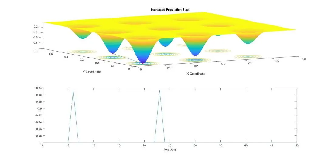
Now the minimum value is always falling at two peaks.

In the bottom plot, we can see the minimum function value ranges between -0.84 and -1.

Now, In order to get global maxima, we can increase the number of interactions or play with the search bound or we can increase population size.

Let's increase the population size to 300 and re-run the code.

options = optimoptions('ga');
options = optimoptions(options,'PopulationSize',300);

tic

for i = 1:num_iteration
    [inputs, fval(i)] = ga(@stalagmite, 2, [], [], [], [], [0;0],[1;1], [], [], options);
    xval(i) = inputs(1);
    yval(i) = inputs(2);
end

run_time_study_3 = toc

figure(3)             
subplot(2,1,1)        
hold on

surfc(x,y,f)          
shading interp        

plot3(xval,yval,fval,'marker','o','markersize',5,'markerfacecolor','r') 
xlabel('X-Coordinate')
ylabel('Y-Coordinate')
title('Increased Population Size')
subplot(2,1,2)       
plot(fval)           
xlabel('Iterations')

Output:

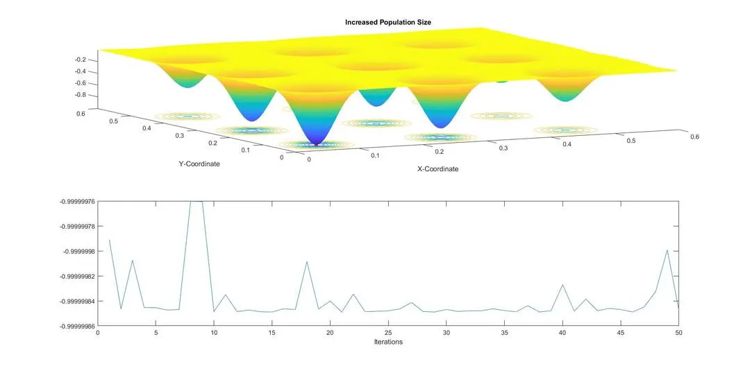
With increased population size we can see now Solver is predicting only a single point and that is our global maxima. We can also see in the bottom plot the maxima value of the function is 0.99 or approx. to 1 and the change with the iteration is almost negligible.

Location of Global Maximum is:-

x = 0.0668

y = 0.0668