Curve fitting using MATLAB

Objective

Write code to fit a linear and cubic polynomial for the Cp data using MATLAB.

Plot the linear and cubic fit curves along with the raw data points of cp vs Temperature.

Write a code to show split wise method to make a better fit of the polynomial curve.

Explain the parameters used to measure the fitness characteristics for both the curves.

Inputs

Data of Specific Heat Capacity values for different temperature is given as input file naming "data".

Solution

Specific Heat Capacity vs Temperature is plotted by loading the given data file in MATLAB to study the variation of cp with respect to temperature.

Using the 'polyfit' function linear and cubic polynomial coefficients are calculated.

Using those coefficients we can form a linear and cubic curve of cp for different temperatures value.

For the different values of temperatures, linear and cubic polynomial equations are used to calculate cp value corresponding to the linear and cubic curve using 'polyval' command.

Then, cp calculated using a linear and cubic curve, input cp is plotted for given temperatures value.

Here is the MATLAB code for that.

clc
clear all
close all

%data preperation

cp_data = load('data');
temperature = cp_data(:,1);
cp = cp_data(:,2);

%curve fitting

% cp = a*T^2 + b*T + c 
% we need to figure out value of a and b such that it fits our curve with least error

linear_coeffs = polyfit(temperature,cp,1);     %calculating linear curve equation coefficients
cubic_coeffs  = polyfit(temperature,cp,3);     %calculating cubic curve equation coefficients

predicted_cp_linear = polyval(linear_coeffs, temperature); %calculating cp based on linear equation
predicted_cp_cubic = polyval(cubic_coeffs, temperature);  %calculating cp based on cubic equation

%plotting and comparing the curve fit with original data

plot(temperature,cp,'linewidth',3)
hold on
plot(temperature,predicted_cp_linear,'linewidth',3,'color','r')   %linear curve plot
plot(temperature,predicted_cp_cubic,'linewidth',3,'color','k')    %cubic curve plot
xlabel('Temperature [K]')
ylabel('Specific Heat Capacity [KJ/Kmol-K]')    
legend('Original Data Set','Linear Curve','Cubic Curve')
legend('Location','northwest')

CODE OUTPUT

Plot temperature vs Actual cp and Curve fitted cp

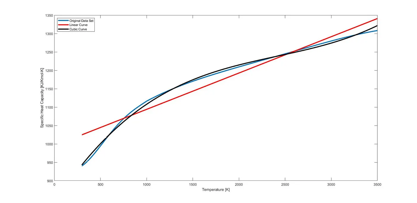
By a visual inspection, we can see a cubic polynomial curve fits better to the input curve than the linear polynomial curve but still cubic curve does not fit perfectly to the original corve.

Using mathematical expression we can calculate the fitness of the curve as explained below.

Parameters to measure the fitness characteristics for the curves

We will calculate the sum of the squares to measure the fitness of the curves. The Sum of squares is a statistical technique used in regression analysis to determine the dispersion of data points. It can be used to determine how well a data series can be fitted to a function. The Sum of squares is used as a mathematical way to find the function that best fits(varies least) from the given data.

There are three terms,. The sum of squares total(SST), the sum of squares regression(SSR), and the sum of squares error(SSE).

Sum of squares total (SST)

It is a variation of the values of a dependent variable from the mean of the dependent variable. The total sum of squares quantifies the total variation in a sample. It is the squared differences between the observed dependent variable and its mean.

`SST = SSR + SSE`

Sum of squares regression(SSR)

The regression sum of squares describes how well a regression model represents the modeled data. A higher regression sum of squares indicates that the model does not fit the data well. It is the sum of the differences between the predicted value and the mean of the dependent variable.

`SSR = sum_(i=1)^n (haty_i - bary)^2`

ŷ_i – the value estimated by the regression line

ȳ – the mean value of a sample

Sum of squares error(SSE)

It is the error in the difference between the observed value and the predicted value. We want to minimize SSE. The smaller the error, the better the estimation power of the regression.

`SSE = sum_(i=1)^n (y_i - haty_i)^2`

y_i – the observed value

ŷ_i – the value estimated by the regression line

If SSE is zero, then SST = SSR. Meaning our regression model captures all the observed variability and is perfect.

The R-squared

This statistic measures how successful the fit is in explaining the variation of the data. R-square can take on any value between 0 and 1, with a value closer to 1 indicating a better fit. For example, an R² value of 0.8234 means that the fit explains 82.34% of the total variation in the data about the average.

An R-squared value above 0.95 shows the good fit of the curve.

`R^2 = (SSR)/(SST)`

CODE for the Fitness Characteristics for the linear and cubic curve

%calculating fitness characteristics.

% By evaluating total sum of squares, regression sum of squares, and residual sum of squares
% We can analyze the fitness of the curve.

%LINEAR CURVE

error_L = (cp - predicted_cp_linear);
error_avg_L = mean(error_L.^2);
SSE_L = sum(error_L.^2);              %SUM OF SQUARE DUE TO ERROR

SSR_L = sum((predicted_cp_linear - mean(cp)).^2); %SUM OF SQUARE OF REGRESSION

SST_L = (SSR_L + SSE_L); %SUM OF SQUARE OF TOTAL

R_squared_L = (SSR_L/SST_L);  %How well the fit curve is explaining the variation of data
R_percentage_L = R_squared_L*100;
Linear_Character = table(error_avg_L,SSE_L,SSR_L,SST_L,R_squared_L,'VariableNames',{'ERROR','SSE','SSR','SST','R_sq'})

if R_squared_L > 0.95
    fprintf("Linear Curve predicts the %.2f percent variation of real curve.",R_percentage_L)
else
    disp("Linear Curve does not predicts the variation of actual curve well")
end
%CUBIC CURVE

error_C = (cp - predicted_cp_cubic);
error_avg_C = mean(error_C.^2);
SSE_C = sum(error_C.^2);              %SUM OF SQUARE DUE TO ERROR

SSR_C = sum((predicted_cp_cubic - mean(cp)).^2); %SUM OF SQUARE OF REGRESSION

SST_C = (SSR_C + SSE_C); %SUM OF SQUARE OF TOTAL

R_squared_C = (SSR_C/SST_C);  %How well the fit curve is explaining the variation of data
R_percentage_C = R_squared_C*100;
Cubic_Character = table(error_avg_C,SSE_C,SSR_C,SST_C,R_squared_C,'VariableNames',{'ERROR','SSE','SSR','SST','R_sq'})
if R_squared_C > 0.95
    fprintf("Cubic Curve predicts the %.2f percent variation of the real curve.",R_percentage_C)
else
    disp("Linear Curve does not predicts the variation of actual curve well")
end

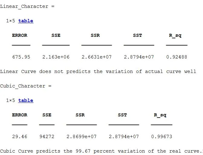
OUTPUT

Conclusion

The R_squared value for the linear curve is 0.92. Linear Curve is able to capture a 92 % variation of the actual curve.

The R_squared value for the cubic curve is 0.99. Cubic Curve is able to capture a 99 % variation of the actual curve.

Split wise method to make a better fit of the Cubic curve

By splitting the temperature and specific heat capacity in a set of a smaller array of 400 columns & calculating polynomial coefficients of those smaller arrays will help in improving the fit of the curve.

The smaller range of the array will lead to a better curve fit.

Now we have split temperature and cp in a smaller set of 8 arrays, each of them containing 400 rows.

Then we have calculated the coefficients of the cubic polynomial for each set of arrays
Then we have predicted cp value via fit curves for all of those corresponding polynomials.

In this way, we have obtained 8 arrays of calculated cp value which we can combine and store in a single big array.

Then that big array is used to plot calculated cp via cubic split wise polynomial fit vs temperature.

Fitness characteristics are also calculated for the split wise cubic curve.

MATLAB CODE

clc
clear all
close all

%data preperation

cp_data = load('data');
temperature = cp_data(:,1);
cp = cp_data(:,2);

%splitwise method
%splitting the temperature and specific heat capacity in a set of smaller array of 400 rows.
%calculating polynomial coefficients of those smaller arrays
%smaller range of array will lead to better curve fit

%splitting temp and cp, calculating coeff and 
%predicted cp value via fit curves for the smaller range

temp_01 = temperature(1:400);  
cp_01 = cp(1:400);
coeffs_01  = polyfit(temp_01,cp_01,3);
predicted_cp_01 = polyval(coeffs_01, temp_01);

temp_02 = temperature(401:800);
cp_02 = cp(401:800);
coeffs_02  = polyfit(temp_02,cp_02,3);
predicted_cp_02 = polyval(coeffs_02, temp_02);

temp_03 = temperature(801:1200);
cp_03 = cp(801:1200);
coeffs_03  = polyfit(temp_03,cp_03,3);
predicted_cp_03 = polyval(coeffs_03, temp_03);

temp_04 = temperature(1201:1600);
cp_04 = cp(1201:1600);
coeffs_04  = polyfit(temp_04,cp_04,3);
predicted_cp_04 = polyval(coeffs_04, temp_04);

temp_05 = temperature(1601:2000);
cp_05 = cp(1601:2000);
coeffs_05  = polyfit(temp_05,cp_05,3);
predicted_cp_05 = polyval(coeffs_05, temp_05);

temp_06 = temperature(2001:2400);
cp_06 = cp(2001:2400);
coeffs_06  = polyfit(temp_06,cp_06,3);
predicted_cp_06 = polyval(coeffs_06, temp_06);

temp_07 = temperature(2401:2800);
cp_07 = cp(2401:2800);
coeffs_07  = polyfit(temp_07,cp_07,3);
predicted_cp_07 = polyval(coeffs_07, temp_07);

temp_08 = temperature(2801:3200);
cp_08 = cp(2801:3200);
coeffs_08  = polyfit(temp_08,cp_08,3);
predicted_cp_08 = polyval(coeffs_08, temp_08);

predicted_cp = [predicted_cp_01;predicted_cp_02;predicted_cp_03;predicted_cp_04;predicted_cp_05;predicted_cp_06;predicted_cp_07;predicted_cp_08];

plot(temperature,predicted_cp,'linewidth',3,'color','y')
hold on
plot(temperature,cp,'linewidth',3)
plot(temperature,cp,'linewidth',3,'color','b')
xlabel('Temperature [K]')
ylabel('Specific Heat Capacity [KJ/Kmol-K]')    
legend('split Curve','Original Data Set')
legend('Location','northwest')

%calculating fitness characteristics.

error = (cp - predicted_cp);
error_avg = mean(error.^2);
SSE = sum(error.^2);              %SUM OF SQUARE DUE TO ERROR

SSR = sum((predicted_cp - mean(cp)).^2); %SUM OF SQUARE OF REGRESSION

SST = (SSR + SSE); %SUM OF SQUARE OF TOTAL

R_squared = (SSR/SST);  %How well the fit curve is explaining the variation of data
R_percentage = R_squared*100;
Cubic_Character = table(error_avg,SSE,SSR,SST,R_squared,'VariableNames',{'ERROR','SSE','SSR','SST','R_sq'})

if R_squared > 0.95
    fprintf("Split Wise Cubic Curve predicts the %0.f percent variation of real curve.",R_percentage)
else
    disp("Split Wise Cubic Curve does not predicts the variation of actual curve well")
end

OUTPUT

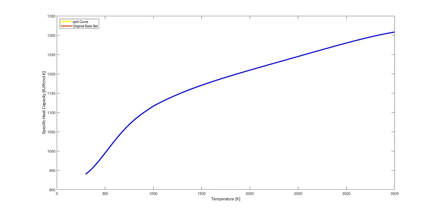
By a visual inspection, we can see a split wise cubic polynomial curve fits perfect to the input curve.

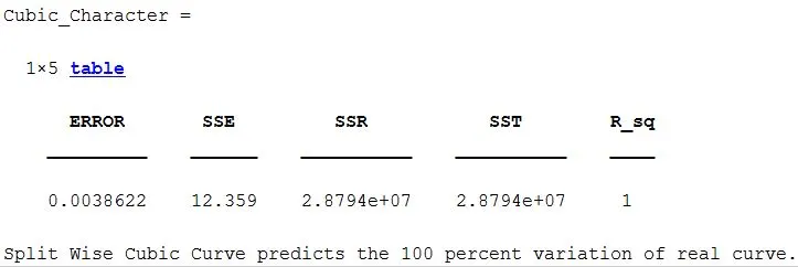
R_squared value is 1 meaning the Split-wise cubic curve captures the 100 % variation of the actual curve. It's the best fit in this case.

Let's define the BEST & PERFECT FIT.

PERFECT FIT

How to make a curve fit perfectly?

To make a curve fit perfect the error estimates should be considered. The perfect fit is a fit where it should match the original curve and shouldn't have any scaling and centering errors in that particular degree of the polynomial. The R^2 value must be equal to 1 and SSE=0.

BEST FIT

How to get the best fit?

A perfect fit can all the time be the best fit but the best fit may not be always a perfect fit. There are basically two methods to obtain the best fit.

1. To increase the degree of the polynomial.
2. To use the split-wise method i.e to split the data into folds and do the curve fitting for it.