Week 3 - Taylor table method and Matlab code

Taylor Table Method and MATLAB Code

Aim:

Derive the fourth order apporximation for Skewed Right Approximation, Skewed Left Approximation and Central difference scheme and write a MATLAB code for the same to evaluate second order derivative of `e^x*cos(x)`.

Taylor Series expansion for Skewed Right Sided Approximation:

Since the numerical stencil is not symmetric the scheme is termed as skewed and we are dealing with 4th order accuracy for which we will need five nodes to the right of the `i^(th)`node

`f(i) = f(i)`

`f(i+1)=f(i) +(Deltax)/(1!)*f'(i)+(Deltax^2)/(2!).f''(i)+(Deltax^3)/(3!).f'''(i)+(Deltax^4)/(4!).f''''(i)+(Deltax^5)/(5!).f'''''(i)+H.O.T`

`f(i+2)=f(i) +(2*Deltax)/(1!)*f'(i)+((2*Deltax)^2)/(2!).f''(i)+((2*Deltax)^3)/(3!).f'''(i)+((2*Deltax)^4)/(4!).f''''(i)+((2*Deltax)^5)/(5!).f'''''(i)+H.O.T`

`f(i+3)=f(i) +(3*Deltax)/(1!)*f'(i)+((3*Deltax)^2)/(2!).f''(i)+((3*Deltax)^3)/(3!).f'''(i)+((3*Deltax)^4)/(4!).f''''(i)+((3*Deltax)^5)/(5!).f'''''(i)+H.O.T`

`f(i+4)=f(i) +(4*Deltax)/(1!)*f'(i)+((4*Deltax)^2)/(2!).f''(i)+((4*Deltax)^3)/(3!).f'''(i)+((4*Deltax)^4)/(4!).f''''(i)+((4*Deltax)^5)/(5!).f'''''(i)+H.O.T`

`f(i+5)=f(i) +(5*Deltax)/(1!)*f'(i)+((5*Deltax)^2)/(2!).f''(i)+((5*Deltax)^3)/(3!).f'''(i)+((5*Deltax)^4)/(4!).f''''(i)+((5*Deltax)^5)/(5!).f'''''(i)+H.O.T`

For the above equations the LHS and RHS are multiplied with a,b,c,d,e,g and for simplicity in terms of representation only the RHS is shown below;

`a*f(i)`

`b*f(i+1)`

`c*f(i+2)`

`d*f(i+3)`

`e*f(i+4)`

`g*f(i+5)`

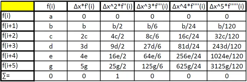
From the above representation we can see that there are 6 unknowns to which there are 6 equations shown below;

`a+b+c+d+e+g=0`

`0+b+2c+3d+4e+5g=0`

`0+b/2+4/2c+9/2d+16/2e+25/2g=1`

`0+b/6+8/6c+27/6d+64/6e+125/6g=0`

`0+b/24+16/24c+81/21d+256/24e+625/24g=0`

`0+b/120+32/120c+243/120d+1024/120e+3125/120g=0`

And the above equations in the form a Matrix to solve for the coefficients can be written as;

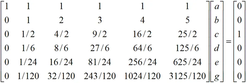
This matrix is computed in the function created to compute skewed right sided approximation absolute error with that of analytical solution. Following this it is better to establish all the facts on to the main equation second order equation to which we are numerically solving.

Dividing both LHS and RHS by `Deltax^2`

`(del^2f)/(delx^2) = (af(i)+bf(i+1)+c*f(i+2)+d*f(i+3)+e*f(i+4)+g*f(i+5))/(delx^2)+O*(Deltax^4)[text(truncation error)]`

As mentioned in the hint, we can show that;

The order of accuracy P = Number of nodes in the stencil N - order of derivative Q

where, N = 6 & Q=2, therefore the order of accuracy P will be 4 as derived above

MATLAB code for Skewed Right Sided Approximation:

%% Skewed left Approximation of 4th order for a 2nd order derivative
function abs_error_SRA = SRA(x,dx)

% analytical function 
f = @(x) exp(x)*cos(x);
% as illustrated in the theory, five equations are needed for computing the
% coefficients a,b,c,d,e and they are stored in the eq1,eq2,eq3,eq4,eq5,eq6
syms a b c d e g
% directories and then recalled in the 'solve' command to compute the
% coeffcients 
eq1 = a + b + c + d + e + g == 0;
eq2 = b + 2*c + 3*d + 4*e + 5*g == 0;
eq3 = b/2 + 4*c/2 + 9*d/2 + 16*e/2 + 25*g/2 == 1;
eq4 = b/6 + 8*c/6 + 27*d/6 + 64*e/6 + 125*g/6 == 0;
eq5 = b/24 + 16*c/24 + 81*d/24 + 256*e/24 + 625*g/24 == 0;
eq6 = b/120 + 32*c/120 + 243*d/120 + 1024*e/120 + 3125*g/120 == 0;


% calling the 'solve command'
Sol = solve([eq1,eq2,eq3,eq4,eq5,eq6],[a,b,c,d,e,g]);
% from the above simplification extracting the coefficients from "Sol"
a = Sol.a;
b = Sol.b;
c = Sol.c;
d = Sol.d;
e = Sol.e;
g = Sol.g;
E = [a;b;c;d;e;g];
disp('Skewed Right Approximation Coefficients')
disp(E)
% the coefficients are placed into the Taylor's series expansion
SRA = (a*f(x) + b*f(x+dx)+ c*f(x+(2*dx)) + d*f(x+(3*dx)) + e*f(x+(4*dx)) + g*f(x+(5*dx)))/(dx^2);

% this functions motive is to give the abs error and to compute it the
% analytically derived solution is needed
ana_deriv = -2*exp(x)*sin(x);
% computed error is plotted, for which user needs to specify the limits of
% "x" and "dx"
abs_error_SRA = abs(SRA - ana_deriv);
end

Taylor Series expansion for Skewed Left Sided Approximation:

Since the numerical stencil is not symmetric the scheme is termed as skewed and we are dealing with 4th order accuracy for which we will need five nodes to the left of the `i^(th)`node

`f(i-5)=f(i) -(5*Deltax)/(1!)*f'(i)+((5*Deltax)^2)/(2!).f''(i) - ((5*Deltax)^3)/(3!).f'''(i) + ((5*Deltax)^4)/(4!).f''''(i) - ((5*Deltax)^5)/(5!).f'''''(i) + ((5*Deltax)^6)/(6!).f''''''(i)+H.O.T`

`f(i-4)=f(i) + (4*Deltax)/(1!)*f'(i)+((4*Deltax)^2)/(2!).f''(i) + ((4*Deltax)^3)/(3!).f'''(i) + ((4*Deltax)^4)/(4!).f''''(i) + ((4*Deltax)^5)/(5!).f'''''(i) + ((4*Deltax)^6)/(6!).f''''''(i)+H.O.T`

`f(i-3)=f(i) -(3*Deltax)/(1!)*f'(i)+((3*Deltax)^2)/(2!).f''(i) - ((3*Deltax)^3)/(3!).f'''(i) + ((3*Deltax)^4)/(4!).f''''(i) - ((3*Deltax)^5)/(5!).f'''''(i) + ((3*Deltax)^6)/(6!).f''''''(i)+H.O.T`

`f(i-2)=f(i) -(2*Deltax)/(1!)*f'(i)+((2*Deltax)^2)/(2!).f''(i) - ((2*Deltax)^3)/(3!).f'''(i) + ((2*Deltax)^4)/(4!).f''''(i) - ((2*Deltax)^5)/(5!).f'''''(i) + ((2*Deltax)^6)/(6!).f''''''(i)+H.O.T`

`f(i-1)=f(i) -(Deltax)/(1!)*f'(i)+((Deltax)^2)/(2!).f''(i) - ((Deltax)^3)/(3!).f'''(i) + ((Deltax)^4)/(4!).f''''(i) - ((Deltax)^5)/(5!).f'''''(i) + ((Deltax)^6)/(6!).f''''''(i)+H.O.T`

`f(i) = f(i)`

Now the coefficeints that are being multiplied are shown below and only the LHS part of the equation is shown, however the same coefficients are multiplied to the RHS as well;

`k*f(i-5)`

`l*f(i-4)`

`m*f(i-3)`

`n*f(i-2)`

`o*f(i-1)`

`p*f(i)`

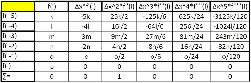
From Taylor's Table we can write;

`text(k+l+m+n+o+p) = 0`

`-5k-4l-3m-2n-o = 0`

`25/2k+16/2l+9/2m+4/2n+o/2 = 1`

`-125/6k-34/6l-27/6m-8/6n-o/6=0`

`625/24k+256/24l+81/24m+16/24n+o/24=0`

`-3125/120k-1024/120l-243/120m-32/120n-o/120=0`

And the above equations in the form a Matrix to solve for the coefficients can be written as;

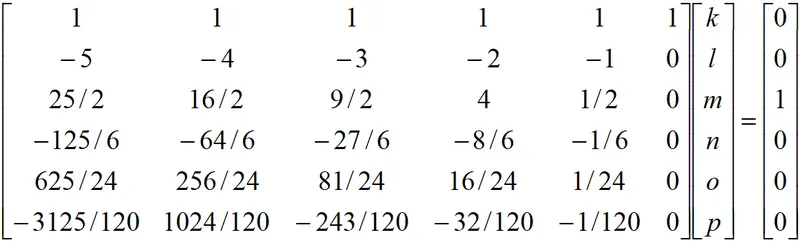
This matrix is computed in the function created to compute skewed left sided approximation absolute error with that of analytical solution. Following this it is better to establish all the facts on to the main equation second order equation to which we are numerically solving.

Dividing both LHS and RHS by `Deltax^2`

`(del^2f)/(delx^2) = (kf(i-5)+lf(i-4)+mf(i-3)+nf(i-2)+of(i-1)+pf(i))/(delx^2)+O*(Deltax^4)[text(truncation error)]`

As mentioned in the hint, we can show that;

The order of accuracy P = Number of nodes in the stencil N - order of derivative Q

where, N = 6 & Q=2, therefore the order of accuracy P will be 4 as derived above

MATLAB code for Skewed Left Approximation function:

%% Skewed left Approximation of 4th order for a 2nd order derivative
function abs_error_SLA = SLA(x,dx)

% analytical function 
f = @(x) exp(x)*cos(x);
% as illustrated in the theory, five equations are needed for computing the
% coefficients a,b,c,d,e and they are stored in the e1,e2,e3,e4,e5
syms k l m n o p
% directories and then recalled in the 'solve' command to compute the
% coeffcients 
eq1 = k + l + m + n + o + p == 0;
eq2 = -5*k - 4*l - 3*m - 2*n - o == 0;
eq3 = 25*k/2 + 16*l/2 + 9*m/2 + 4*n/2 + o/2 == 1;
eq4 = -125*k/6 -64*l/6 - 27*m/6 - 8*n/6 - o/6 == 0;
eq5 = 625*k/24 + 256*l/24 + 81*m/24 + 16*n/24 + o/24 == 0;
eq6 = -3125*k/120 - 1024*l/120 - 243*m/120 - 32*n/120 - o/120 == 0;

% calling the 'solve command'
Sol = solve([eq1,eq2,eq3,eq4,eq5,eq6],[k,l,m,n,o,p]);
% from the above simplification extracting the coefficients from "Sol"
k = Sol.k;
l = Sol.l;
m = Sol.m;
n = Sol.n;
o = Sol.o;
p = Sol.p;
F = [k;l;m;n;o;p];
disp('Skewed Left Approximation Coefficients')
disp(F)
% the coefficients are placed into the Taylor's series expansion
SLA = (k*f(x-(5*dx))+ l*f(x-(4*dx)) + m*f(x-(3*dx)) + n*f(x-(2*dx))+ o*f(x-dx) + p*f(x))/(dx^2);

% this functions motive is to give the abs error and to compute it the
% analytically derived solution is needed
ana_deriv = -2*exp(x)*sin(x);
% computed error is plotted, for which user needs to specify the limits of
% "x" and "dx"
abs_error_SLA = abs(SLA - ana_deriv);
end

Taylor Series expansion for CDS:

Since the numerical stencil is symmetric the scheme and we are dealing with 4th order accuracy for which we will need four nodes one to the right , one to the left and the other two top and bottom of the `i^(th)`node

`f(i-2)=f(i) -(2*Deltax)/(1!)*f'(i)+((2*Deltax)^2)/(2!).f''(i)-((2*Deltax)^3)/(3!).f'''(i)+((2*Deltax)^4)/(4!).f''''(i)+H.O.T`

`f(i-1)=f(i) -(Deltax)/(1!)*f'(i)+(Deltax^2)/(2!).f''(i)-(Deltax^3)/(3!).f'''(i)+(Deltax^4)/(4!).f''''(i)+H.O.T`

`f(i) = f(i)`

`f(i+1)=f(i) +(Deltax)/(1!)*f'(i)+(Deltax^2)/(2!).f''(i)+(Deltax^3)/(3!).f'''(i)+(Deltax^4)/(4!).f''''(i)+H.O.T`

`f(i+2)=f(i) +(2*Deltax)/(1!)*f'(i)+((2*Deltax)^2)/(2!).f''(i)+((2*Deltax)^3)/(3!).f'''(i)+((2*Deltax)^4)/(4!).f''''(i)+H.O.T`

Now the coefficeints that are being multiplied are shown below and only the LHS part of the equation is shown, however the same coefficients are multiplied to the RHS as well;

`p * f(i-2)`

`q * f(i-1)`

`r * f(i)`

`s * f(i+1)`

`t * f(i+2)`

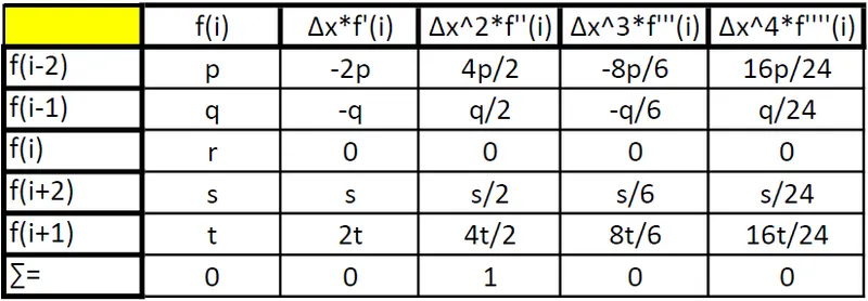
From Taylor Table the following equation can be written;

`p + q+r+s+t=0`

`-2p-q+0+s+2t=0`

`2p+q/2+0+s/2+2t=1`

`-8/6p-q/6+s/6+8/6t=0`

`16/24p+q/24+0+s/24+16/24t=0`

As indicated in the above problem statement, the same can be converted into appropriate matrix format to solve for the coefficients;

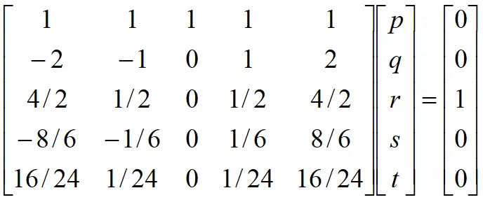
This matrix is computed in the function created to compute central difference absolute error with that of analytical solution. Following this it is better to establish all the facts on to the main equation second order equation to which we are numerically solving.

Dividing both LHS and RHS by `Deltax^2`

`(del^2f)/(delx^2) = (p*f(i-2)+q*f(i-1)+r*f(i)+s*f(i+1)+t*f(i+2))/(delx^2)+O*(Deltax^4)[text(truncation error)]`

solution becomes fairly simple, there are 5 unkowns and there are 5 equations.

As mentioned in the hint, we can show that;

The order of accuracy P = Number of nodes in the stencil N - order of derivative Q + 1

where, N = 5 & Q=2, therefore the order of accuracy P will be 4 as derived above

MATLAB function for Central Difference Scheme:

%% Central Difference Scheme of 4th order approximation 

function abs_error_CDS = CDS(x,dx)

% analytical function 
f = @(x) exp(x)*cos(x);
% as illustrated in the theory, five equations are needed for computing the
% coefficients a,b,c,d,e and they are stored in the eq1,eq2,eq3,eq4,eq5
syms p q r s t
% directories and then recalled in the 'solve' command to compute the
% coeffcients 
eq1 = p + q + r + s + t == 0;
eq2 = -2*p - q + s + 2*t == 0;
eq3 = 4*p/2 + q/2 + s/2 + 4*t/2 == 1;
eq4 = -8*p/6 - q/6 + s/6 + 8*t/6 == 0;
eq5 = 16*p/24 + q/24 + s/24 + 16*t/24 == 0;



% calling the 'solve command'
Sol = solve([eq1,eq2,eq3,eq4,eq5],[p,q,r,s,t]);
% from the above simplification extracting the coefficients from "Sol"
p = Sol.p;
q = Sol.q;
r = Sol.r;
s = Sol.s;
t = Sol.t;
D = [p;q;r;s;t];
disp('CDS Coefficients')
disp(D)
% the coefficients are placed into the Taylor's series expansion
CDS = (p*f(x-(2*dx))+ q*f(x-dx)+ r*f(x)+ s*f(x+dx) + t*f(x+(2*dx)))/(dx^2);

% this functions motive is to give the abs error and to compute it the
% analytically derived solution is needed
ana_deriv = -2*exp(x)*sin(x);
% computed error is plotted, for which user needs to specify the limits of
% "x" and "dx"
abs_error_CDS = abs(CDS - ana_deriv);
end

The above three functions need to be called and results must be plotted for the same:

Main Program:

%% Clear workspace 
clear all
close all
clc
%% Specifying the intervals and step size 
x  = pi/3;
dx = linspace(pi/4,pi/4000,100);
% alloting matrix to speed up the process
SLA_error = zeros(1,length(dx)); 
SRA_error = zeros(1,length(dx));
CDS_error = zeros(1,length(dx));
FDA_error = zeros(1,length(dx));
BDA_error = zeros(1,length(dx));
%% Loop to compute error for values of dx
for i = 1 : length(dx)
    
    SLA_error(i) = SLA(x,dx(i));
    SRA_error(i) = SRA(x,dx(i));
    CDS_error(i) = CDS(x,dx(i));
    FDA_error(i) = FDS_func(x,dx(i));
    BDA_error(i) = BDS_func(x,dx(i));
end

%% Plot error against dx 
figure(1)
loglog(dx,SLA_error,'-xb')
grid on
hold on 
loglog(dx,SRA_error,'-pr')
grid on
hold on 
loglog(dx,CDS_error,'-+g')
grid on
hold on
loglog(dx,FDA_error,'-*k')
grid on
hold on
loglog(dx,BDA_error,'-*m')
grid on
hold on
xlabel('dx')
ylabel('Absolute Error')
legend('Skewed Left Approximation','Skewed Right Approximation','Central difference Scheme','Forward Difference Approximation','Backward Difference Approximation','Location','northwest')
title('Comparison Plot: First order and fourth order')
saveas(gca,'dx vs Approximation.jpg')
%% To estimate the slope of the curve using the "gradient" command
% converting the numerical points into a log line
s1 = log10(dx);
s2 = log10(SLA_error);
s3 = log10(SRA_error);
s4 = log10(CDS_error);
% to get the gradient 
grad_1 = gradient(s2,s1); % slope for SLA
grad_2 = gradient(s3,s1); % slope for SRA
grad_3 = gradient(s4,s1); % slope for CDS
% the gradient can be observed by plotting
figure(2)
plot(grad_1,'b:x')
grid on
hold on
plot(grad_2,'r--*')
grid on
hold on
plot(grad_3,'g-o')
legend('Skewed Left Approximation','Skewed Right Approximation','Central Difference Scheme','Location','northeast') 
title('Slope of the Error Curves')
saveas(gca,'Gradient Plot.jpg')

Results:

Discussions:

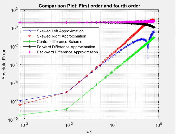
1. The first plot that shows the relationship between first order approximation schemes (both FDS and BDS) and the fourth order differencing schemes. From this we can definitely comment that fourth order is much more accurate and most signifantly indicates that on reducing 'dx' fourth order also approaches solutions solutions at a much faster rate than FDS and BDS.
2. The next course is to compare the three fourth order schemes, and for the same the central differencing scheme tends to show less error than the other other two schemes. This is primarily because the distance of nodes from the 'i th' node is considerably smaller as compared to that of skewed schemes where the nodes are far away that adds to the absolute error. The plotted is in loglog scale in order to compress and easy to interpret the results.
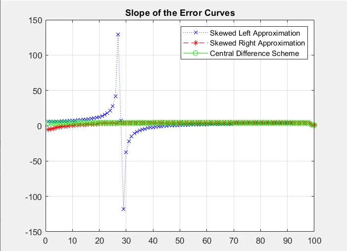
3. Not much perturbation in the results on incrementing 'dx' and the behavior is constant as seen in figure(2) for the the three fourth order schemes and can be concluded that there is no sudden jump in error due to increment in dx.

Why a skewed scheme is useful? What can a skewed scheme do that a central difference scheme cannot do?

When the problem is defined only at one end, the given data can be associated to the left or right end nodes from where the skewed scheme can be applied, unlike the central difference that requires a symmetric numerical stencil. This makes it impossible to use central difference scheme at the boundaries, however, within the domain as the solution progresses further in the flow field the CDS works like a charm.

Now, as discussed above the skewed schemes tend to bring errors that will add up and affect the solution and to keep that in check most solvers using the skewed schemes use optimal low values for 'dx' for stability and consistency.

Inference:

The above exercise takes us through the derivation of fourth order approximations using the Taylor Table method for a second order derivative and compare the results to give an idea of how consistent and accurate is each scheme.