Project 2 - Rankine cycle Simulator

Rankine Cycle Simulation Using Matlab

Aim:

To plot the state points in the Rankine cycle, T-s and h-s graph using the two laws of thermodynamics derived expressions.

Literature Review:

The two laws of thermodynamics have been used to derive the required relations for the Rankine cycle. Thermodynamics that involve phase changes of the working fluid are defined as vapor cycles and these cycles are employed to produce power and they are defined as “Vapor Power Cycles”.

Phase Changes:

The states of the liquid and vapor needs to be clear.

• Near the saturation curve for pure substances

1. Liquid that is about to vaporize is called saturated liquid
2. Vapor that is about to condense is called saturated vapor
3. Between the above states is called saturated liquid-vapor mixture

• Away from the saturation line

1. Liquid that is not about to is called compressed liquid
2. Vapor not about to condense is called superheated vapor

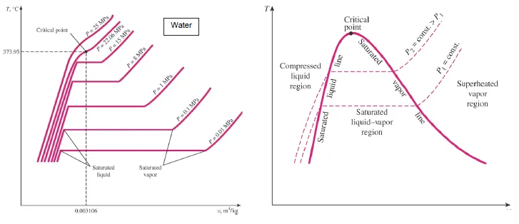
Along with above definitions one must also remember that temperatures and pressures are important properties involved. Phase changes generally occurs near the “saturation temperature” and “saturation pressure”. Another important entity is the “latent heat of vaporization”

When all the above entities are plotted as T-v we get (for water): [1]

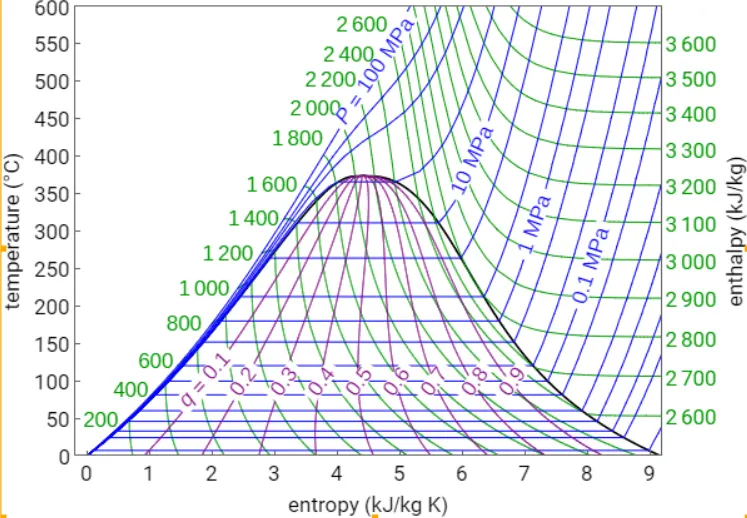
The property is extended to plotting the T-s graph: [2]

Now that the behavior of the phases of the water has been briefly looked into, the same is used to generate electricity. Steam here is used as driver for the turbines to produce run and produce electricity, and this steam power cycle can be approximated to the ideal Rankine Cycle. The schematics below will illustrate the process: [3]

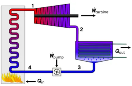
Process

1-2 Isentropic Expansion: Vapor expansion occurs in the turbine, here the quality of the steam will determine the entirety of the stage as the drop in temperature can result in erosion of the blades due to the moisture. Hence, low quality of steam cannot be tolerated; quality must be 90% or above.

2-3 Isobaric Heat Rejection: Here the vapor-liquid mixture is converted to saturated liquid, when this process occurs there are certain difficulties namely the desired quality of the saturated liquid isn’t achieved and it is difficult to design a compressor that can handle two phases.

3-4 Isentropic Compression: The condensate from the previous stage enters the pump and the sole purpose of this stage is to increase the pressure and the work done is small relative the turbine.

4-1 Isobaric Heat Transfer: High pressure condensate enters the boiler and is heated to saturation temperature and further heater to convert it to saturated steam that will enter the turbine.

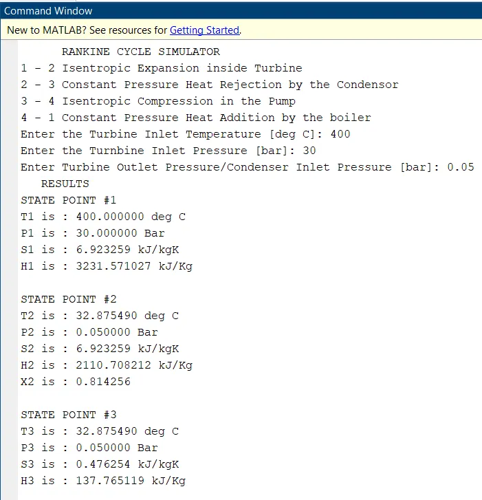
The theory above is used to calculate the values of temperature, pressure and evaluate the state of each point on the Rankine Cycle.

MATLAB Code:

XSteam.m function is used to get the data as seen in the fig:2 for the Rankine_Cycle_Sim.m code to be executed. XSteam.m file has been made available readily and the below code will help realize state points and plot them:

% clear workspace
clear all 
close all
clc

%% Headings that define the Rankine Cycle needs to be Displayed

disp('      RANKINE CYCLE SIMULATOR    ');
disp('1 - 2 Isentropic Expansion inside Turbine');
disp('2 - 3 Constant Pressure Heat Rejection by the Condensor');
disp('3 - 4 Isentropic Compression in the Pump');
disp('4 - 1 Constant Pressure Heat Addition by the boiler');

%% To feed the inputs as specified in the problem 

T1 = input('Enter the Turbine Inlet Temperature [deg C]: ');
P1 = input('Enter the Turnbine Inlet Pressure [bar]: ');
P2 = input('Enter Turbine Outlet Pressure/Condenser Inlet Pressure [bar]: ');

%% Thermodynamic relationships require specific heats viz Cp and Cv both 

% If and when the specific heat is required for dealing with calculations on the
% vapour side of the T-s graph and when the 'x' fraction needs to be
% computed
Cp_Vapour_P1 = XSteam('CpV_p',P1);
Cp_Vapour_P2 = XSteam('CpV_p',P2);
Cv_Vapour_P1 = XSteam('CvV_p',P1);
Cv_Vapour_P2 = XSteam('CvV_p',P2);

% If and when the specific heat is required for dealing with calculations on the
% liquid side of the T-s graph and when the 'x' fraction needs to be
% computed
Cp_Liquid_P1 = XSteam('CpV_p',P1);
Cp_Liquid_P2 = XSteam('CpV_p',P2);
Cv_Liquid_P1 = XSteam('CvV_p',P1);
Cv_Liquid_P2 = XSteam('CvV_p',P2);

% Need the entropy and enthalpy values to calculate the parameters for the
% state points 
% entities that can be extracted using the pressure before turbine inlet
T_1s = XSteam('Tsat_p',P1);
S1 = XSteam('s_pt',P1,T1);
S_1f = XSteam('sL_p',P1);
S_1g = XSteam('sV_p',P1);
S_1fg = (S_1g - S_1f);
H1 = XSteam('h_pt',P1,T1);
H_1f = XSteam('hL_p',P1);
H_1g = XSteam('hV_p',P1);
H_1fg = (H_1g - H_1f);

% entities that can be extracted using the pressure before turbine inlet

T_2s = XSteam('Tsat_p',P2);
S_2f = XSteam('sL_p',P2);
S_2g = XSteam('sV_p',P2);
S_2fg = (S_2g - S_2f);
H_2f = XSteam('hL_p',P2);
H_2g = XSteam('hV_p',P2);
H_2fg = (H_2g - H_2f);

%% Thermodynamic properties that can be calculated using the above values
% s2-s1 = Cv*ln(T2/T1) - R*ln(P2/P1) [change in entropy relation with
% s2-s1 = Cp*ln(T2/T1) + R*ln(V2/V1)  temp and press using laws of TD]
% Wp = h2-h1 = v(p2-p1))             [work done by the pump]
% Wt = h3-h4 for turbine             [work done by the turbine]
% x = (s2-sf)/(sg-sf)                [steam quality 0<x<1; s2>sf ; sf<s2<sg]
% h2 = hg*x + hf*(1-x)= hf + x*hfg   [specific enthalpy]H_2f + X2*H_2fg;
% h2 = h2g*x + Cv*(T2-T_2s)          [specific enthalpy]
% s2 = sf + x*(sg-sf)                [specific entropy]
% n_th = Wt-Wp/Q_in                  [thermal efficiency]
% bwr = Wp/Wt = (h3-h2)/(h8-h1)      [generally less than 1% of power
%                                     developed by the turbine] 

%% Results banner that needs to be displayed before the state points 
disp('   RESULTS   ');

%% State Point #1
disp('STATE POINT #1');
fprintf('T1 is : %f deg C \n',T1)
fprintf('P1 is : %f Bar \n',P1)
fprintf('S1 is : %f kJ/kgK \n',S1)
fprintf('H1 is : %f kJ/Kg \n\n',H1)

%% State Point #2
disp('STATE POINT #2');
S2 = S1;
% to calculate T2 we need the above mentioned thermodynamic relations 
% X2 (dryness fraction) needs to be calculated first 
if (S2<=S_2g)
    X2 = ((S2-S_2f)/S_2fg);
else 
    X2 = 1;
end
% to compute T2
if X2<1
    T2 = T_2s;
else
    T2 = (T_2s + 273.15)*exp((S2-S_2g)/Cv_Vapour_P2);
    T2 = T2-273.15;
end
% to compute H2
if (X2<1)
    H2 = H_2f + X2*H_2fg;
else
    H2 = H_2g + Cv_Vapour_P2*(T2-T_2s);
end

fprintf('T2 is : %f deg C \n',T2)
fprintf('P2 is : %f Bar \n',P2)
fprintf('S2 is : %f kJ/kgK \n',S2)
fprintf('H2 is : %f kJ/Kg \n',H2)
fprintf('X2 is : %f \n\n',X2)


%% State Point #3
disp('STATE POINT #3');

T3 = T_2s;    % this will be the temperature before the condensor
P3 = P2;      % T-s graph the constant pressure line will be plot 
S3 = S_2f;    
H3 = H_2f;
fprintf('T3 is : %f deg C \n',T3)
fprintf('P3 is : %f Bar \n',P3)
fprintf('S3 is : %f kJ/kgK \n',S3)
fprintf('H3 is : %f kJ/Kg \n\n',H3)

%% State Point #4
disp('STATE POINT #4');

S4 = S3;
P4 = P1; % pressure at the pump outlet will be turbine inlet 

% for computing 'T3' 
V3 = XSteam('vL_p',P3);
Wp = V3*(P4-P3)*100; % refer to the above thermodynamic equations
H4 = Wp + H3;        % refer to the above thermodynamic equations
T4 = T_1s/exp((S_1f-S4)/Cp_Liquid_P1);
fprintf('T4 is : %f deg C \n',T4)
fprintf('P4 is : %f Bar \n',P4)
fprintf('S4 is : %f kJ/kgK \n',S4)
fprintf('H4 is : %f kJ/Kg \n\n',H4)

%% Work done and efficiency calculations

% work done by the turbine 
Wt = H1 - H2;
% specific steam consumption
sp_consumption_turbine = 3600 / Wt;
% net work done 
Wnet = Wt - Wp;
% heat input 
Qin = H1 - H4;
% efficiency of the cycle 
n_eff = (Wnet/Qin)*100;
% back work ratio
bwr = Wp/Wt;

fprintf('Work done by Turbine : %f  kJ/kg\n',Wt)
fprintf('Work done by pump : %f  kJ/kg\n',Wp)
fprintf('Net Work done : %f  kJ/kg\n',Wnet)
fprintf('Total Heat Input : %f  kJ/kg\n',Qin)
fprintf('Specific Steam Consumption by Turbine: %f kg/kWh \n',sp_consumption_turbine)
fprintf('Back Work Ratio: %f \n',bwr)
fprintf('Thermal Efficiency: %f ',n_eff);disp('%')

%% Plot T-s using the above data 

% to plot the steam curve 1 to 373 K on the T-s graph and for h-s graph
Temperature = linspace(0,450,1000);
for i = 1:length(Temperature)
    s_Liquid(i) = XSteam('sL_T',Temperature(i));
    s_Vapour(i) = XSteam('sV_T',Temperature(i));
    h_Liquid(i) = XSteam('hL_T',Temperature(i));
    h_Vapour(i) = XSteam('hV_T',Temperature(i));
end

% T-s plot
figure(1)
hold on
plot(s_Liquid,Temperature,'LineWidth',2,'color','r')
plot(s_Vapour,Temperature,'LineWidth',2,'color','r')
hold on
plot([S1 S2],[T1 T2],'LineWidth',1,'color','b')
plot([S2 S_2g],[T2 T_2s],'LineWidth',1,'color','b') 
plot([S_2g S3],[T_2s T3],'LineWidth',1,'color','b')
plot([S3 S4],[T3 T4],'LineWidth',1,'color','b')
plot([S4 S_1f],[T4 T_1s],'LineWidth',1,'color','b')
plot([S_1f S_1g],[T_1s T_1s],'LineWidth',1,'color','b')
plot([S_1g S1],[T_1s T1],'LineWidth',1,'color','b')
hold on
% in this plot the state points needs to be mentioned
text(S1,T1,'1')
text(S2,T2,'2')
text(S_2g,T_2s,'2s')
text(S3,T3,'3')
text(S4,T4,'4')
text(S_1f,T_1s,'4s')
text(S_1g,T_1s,'1s')
hold on
% to show direction of the plot
text(S4,((T3+T4)/2),'\wedge','HorizontalAlignment','center','color','k')
text(((S_1f+S_1g)/2),T_1s,'\rangle','color','k')
text(S1,((T1+T2)/2),'\vee','HorizontalAlignment','center','color','k')
text(((S_2g+S3)/2),T3,'\langle','color','k')
hold on
% labeling the plot 
xlabel('Entropy [kJ/kg-K]','FontSize',12,'FontWeight','bold','color','b')
ylabel('Temperature [K]','FontSize',12,'FontWeight','bold','color','b')
title('Rankine Cycle T-s plot','FontSize',21,'FontWeight','bold','color','k')

%% Plot h-s
% similar steps to be followed here to plot the graph with all the details
figure(2)
hold on 
plot(s_Liquid,h_Liquid,'LineWidth',1.5,'color','r')
plot(s_Vapour,h_Vapour,'LineWidth',1.5,'color','r')
hold on
plot([S1 S2],[H1 H2],'color','g')
text(S1,H1,'1')
plot([S2 S3],[H2 H3],'color','g')
text(S2,H2,'2')
plot([S3 S4],[H3 H4],'color','g')
text(S3,H3,'3')
plot([S4 S1],[H4 H1],'color','g')
text(S4,H4,'4')
hold on
% labeling the plot 
xlabel('Entropy [kJ/kg-K]','FontSize',12,'FontWeight','bold','color','b')
ylabel('Enthalpy [kJ/kg]','FontSize',12,'FontWeight','bold','color','b')
title('Rankine Cycle h-s plot','FontSize',21,'FontWeight','bold','color','k')

%% Save plots in folder
saveas(1,'T-s Diagram.jpg')
saveas(2,'h-s Diagram.jpg')

Plots and Results:

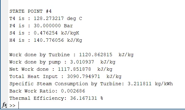
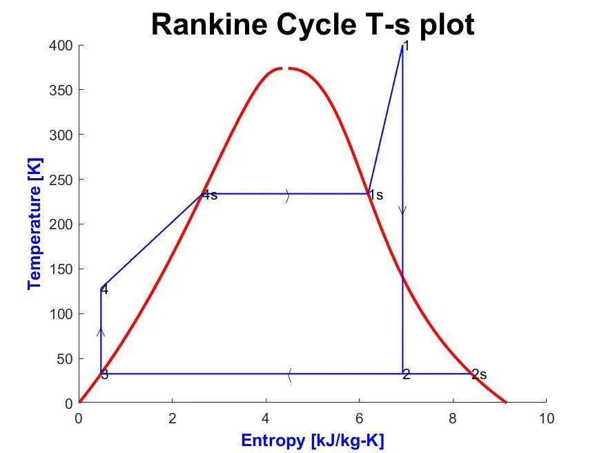
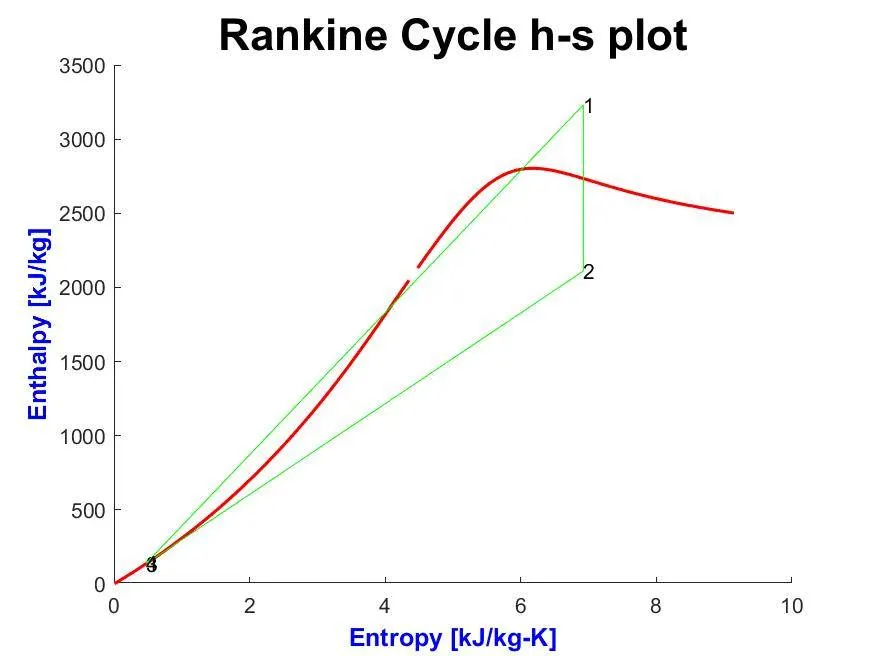
Discussions:

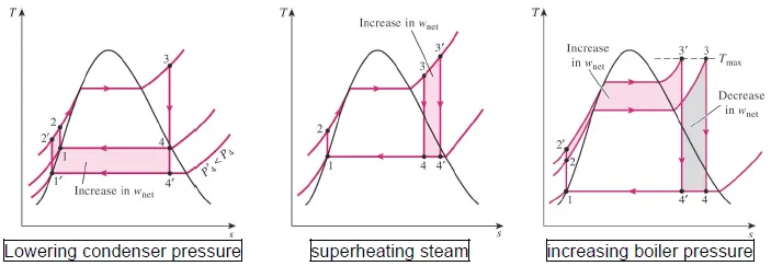
For all practical reasons the efficiency of the cycle is of prime importance, there are a few ways that have been listed.

1. Lowering the condenser pressure
2. Superheating Steam
3. Increasing boiler pressure

Are the cases considered as the way to make modifications to improve the efficiency, they are shown in the below figures using the T-s diagram:

Some of the real time solutions to effectively solve the above shortfalls of the cycle, in real time the below mentioned solutions are used:

1. Ideal Reheated Rankine Cycle:

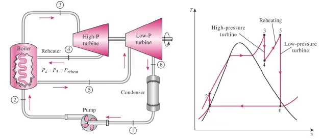
Two stage turbine is used and reheating the steam between the high pressure and low pressure turbine will effectively solve the moisture content.

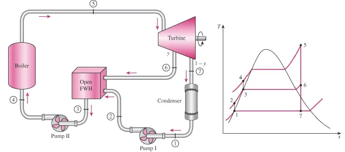
2. Open Feed-water heater (Ideal Regenerative Rankine Cycle): The idea here is to have a mixing chamber is to have steam extracted to get mixed with condensate and this will avoid any thermal shocks in the boiler while reducing the operating costs.

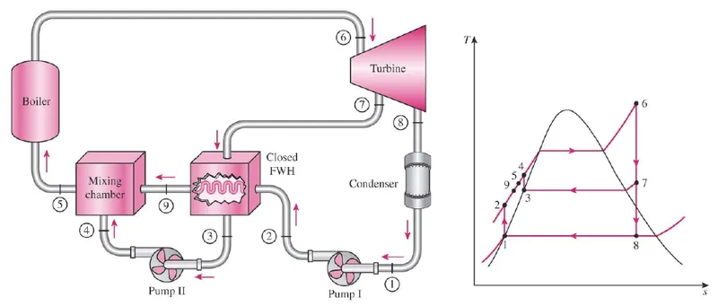
3. Closed Feed-water heater (Ideal Regenerative Rankine Cycle): Similar to the above system, however, in this set up the mixing of the two extract from turbine and condenser pump is not happening directly by using a heat exchanger. If it is observed even though they are at different pressures which is an advantage and the energy balance for the closed feed water heater can be analyzed in an identical manner.

4. Cogeneration and Combined Power cycle:

Here the steam cycles are combined with gas power cycles (seen in fig.9) which gives rise to the term combined cycle. The Cogeneration is a process that involves including a process heater (seen in fig.8) into the Rankine cycle.

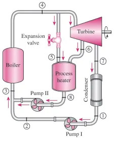
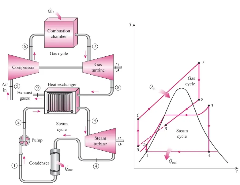
fig.8: Cogeneration fig.9: Combined Power Cycles

Inference:

This exercise threw light on the Rankine Cycle and its processes, including the various methods that could be used to improve the effciency. For the given parameters both the net work output or net work done and the back work ratio was estimated and displayed in the results.