Project 1 - Parsing NASA thermodynamic data

File Parsing

Aim:

To parse data from NASA thermodynamic data file and compute the specific heat, enthalpy, entropy for the gaseous species and plot for the local temperature range for oxygen, nitrogen and carbon dioxide. Also, calculate the molecular weight of the species.

Literature Review:

Parsing: By definition parsing is to resolving into logical syntactic components, or simply splitting the string to smaller usable strings.

Specific Heat [Cp]: defined as the amount of heat required per unit mass to raise its temperature by 1 deg C.

Enthalpy [h]: it is the sum of the internal energy and the product of pressure and volume of a thermodynamic system H = E + PV.

Entropy [s]: it is typically defined by the second law of thermodynamics which concerns with the quality of the energy that is the same amount of energy in different forms can have different potential to be converted to work. So Kelvin-Plank and Clausius proposed their statements that heat cannot be 100% converted to work and transferring heat from cooler body to a hotter body will require external work.

To compute the above properties, the following equations are employed;

Additionally, we have to compute the molecular weight of the species, and the respective atomic weights will be needed for the calculation of molecular weight.

Thermodynamic properties calculation function MATLAB code:

% With reference to the formulae provided in the lecture, they are used to compute the specific
% heat[Cp], entropy[s] and enthalpy[h] for the list of elements in the NASA
% thermodynamic data sheet provided. The data sheet contains the
% coefficients (a1 to a14) required along with the local temperatures 
% For range of temperatures below the local medium tmeperature of each element
% coefficients a8 through a14 are used else a1 to a8 are to be used for the
% calculations, and the same has been created into a function that can be
% called for temperature span of low to high local temperatures.
function [Cp,s,h] = therm_calc_func(a1,a2,a3,a4,a5,a6,a7,a8,a9,a10,a11,a12,a13,a14,loc_med_temp,R,T)

   for i = 1:length(T)
       
         if (T(i)>loc_med_temp)
             Cp = (a1+(a2.*T)+(a3.*(T.^2))+(a4.*(T.^3))+(a5.*(T.^4))).*R;
             h = (a1 + ((a2.*T)./2) + ((a3.*(T.^2))./3) + ((a4.*(T.^3))./4) + ((a5.*(T.^4))./5) + (a6./T)).*R.*T;
             s = ((a1.*log(T)) + (a2.*T) + ((a3.*(T.^2))./2) + (a4.*(T.^3)./3) + ((a5.*(T.^4))./4) + a7).*R;
         else
             Cp = (a8+(a9.*T)+(a10.*(T.^2))+(a11.*(T.^3))+(a12.*(T.^4))).*R;
             h = (a8 + ((a9.*T)./2) + ((a10.*(T.^2))./3) + ((a11.*(T.^3))./4) + ((a12.*(T.^4))./5) + (a13./T)).*R.*T;
             s = ((a8.*log(T)) + (a9.*T) + ((a10.*(T.^2))./2) + ((a11.*(T.^3))./3) + ((a12.*(T.^4))./4) + a14).*R;             
         end
    end
end

• This loop helps to iteratively calculate the specific heat, enthalpy and entropy for each species at the temperature ranges as specified in the data sheet.
• The for loop condition I used to iterate the temperature range, and the if-else condition to selectively use the coefficients from the data sheet.

Main Body to Parse, Plot and Save MATLAB code:

% Clear workspace for file parsing NASA therm data
clear all 
close all
clc

% To read the Thermo data from the directory
f1 = fopen('THERMO.dat','r');

% file heading name is stored and is not important for further calculations
fgetl(f1); 
% The global temperatures are mentioned in this line 
temperature_string = fgetl(f1);
    g_temp = strsplit(temperature_string, ' '); % delimiter in this case is space between each temperature  
         glt = str2num(g_temp{2}); % global low temperature [K]
         gmt = str2num(g_temp{3}); % global medium temperature [K]
         ght = str2num(g_temp{4}); % global high temperature [K]
% Next three lines are to skipped because the text lines start with
% exclamation mark and can be avoided the below syntax can be used
 for i = 1:3
    d = fgetl(f1);
 end
% The 53 species data that are considered for the calculation and plotting
% are stored in the lines below, a 'for' loop can be constructed to read the
% and record the required for each species and repeat the same again for
% the next species. 

for i = 1:53
    % first line for each species contains the name of species and the three local temperatures 
    species_header = fgetl(f1)
    x = strsplit(species_header,' '); % once again using space between each as delimiter
        
        species_name = (x{1}); % here the string can remain as is and need not be converted into values
        y = length(x); % defining the positions for each individual strings makes it easy to isolate 
        % to extract the local temperatures
        loc_low_temp = str2double(x{y-3}); % the cell charaters are converted to double precision values [K]
        loc_med_temp = str2double(x{y-1}); % [K]
        loc_high_temp= str2double(x{y-2}); % [K]

% moving to the next line to extract coefficients a1 to a5
        coeff_line1 = fgetl(f1); 
% the coefficients can be identified using the string find command and
% stored individully 
        z = strfind(coeff_line1,'E'); % this will identify the 'E' in the line and stores the positions
        a1 = str2double(coeff_line1(1:z(1)+3));
        a2 = str2double(coeff_line1(z(1)+4:z(2)+3));
        a3 = str2double(coeff_line1(z(2)+4:z(3)+3));
        a4 = str2double(coeff_line1(z(3)+4:z(4)+3));
        a5 = str2double(coeff_line1(z(4)+4:z(5)+3));

% jumping to the nex line to get the a6 to a a10 coefficients 
        coeff_line2 = fgetl(f1);
% to identify and store the coefficients from the string
        z_1 = strfind(coeff_line2,'E'); % this will identify the 'E' in the line and stores the positions
        a6 = str2double(coeff_line2(1:z_1(1)+3));
        a7 = str2double(coeff_line2(z_1(1)+4:z_1(2)+3));
        a8 = str2double(coeff_line2(z_1(2)+4:z_1(3)+3));
        a9 = str2double(coeff_line2(z_1(3)+4:z_1(4)+3));
        a10 = str2double(coeff_line2(z_1(4)+4:z_1(5)+3));

% jumping to the nex line to get the a11 to a a14 coefficients
        coeff_line3 = fgetl(f1);
% to identify and store the coefficients from the string
        z_2 = strfind(coeff_line3,'E'); % this will identify the 'E' in the line and stores the positions
        a11 = str2double(coeff_line3(1:z_2(1)+3));
        a12 = str2double(coeff_line3(z_2(1)+4:z_2(2)+3));
        a13 = str2double(coeff_line3(z_2(2)+4:z_2(3)+3));
        a14 = str2double(coeff_line3(z_2(3)+4:z_2(4)+3));

% coefficients, temperature are all available to compute the required
% specific heat, enthaply and entropy. Calling the functions below to
% compute
 R = 8.314; % J/mol*K universal constant
 T = linspace(loc_low_temp,loc_high_temp,500);
 [Cp,s,h] = therm_calc_func(a1,a2,a3,a4,a5,a6,a7,a8,a9,a10,a11,a12,a13,a14,loc_med_temp,R,T);
 
% to create a directory to store the plots 

mkdir(['D:\MATLAB\File Parsing\NASA Therm Data Parsing\',species_name]);

% plotting the above the results for each species 
            figure(1) % plot for specific heat 
            plot(T,Cp,'lineWidth',3,'color','c')
            xlabel('Temperature [K]');ylabel('Specific Heat [J/kg-K]')
            title(sprintf('Temperature Vs Specific Heat for %s',species_name))
            figure(2) % plot for enthalpy
            plot(T,h,'lineWidth',3,'color','m')
            xlabel('Temperature [K]');ylabel('Enthalpy [J]')
            title(sprintf('Temperature Vs Enthalpy for %s',species_name))
            figure(3) % plot for entropy
            plot(T,s,'lineWidth',3,'color','r')
            xlabel('Temperature [K]');ylabel('Entropy [J/K]')
            title(sprintf('Temperature Vs Entropy for %s',species_name))
            
            process = (['D:\MATLAB\File Parsing\NASA Therm Data Parsing\',species_name]);
            cd(process)
% the plots needs to be saved, saving in image format '.jpg' in the same
% working directory
        saveas(1,'Specific Heat.jpg')
        saveas(2,'Enthalpy.jpg')
        saveas(2,'Entropy.jpg')

% final step is to compute the molecular weight, it is easy to complete the
% loop with calculation of the molecular weight because we have already
% familiarized with the element that all the above thermodynamic properties
% are being calculated. Finally we can store the value of into a .txt file
% in the same folder for future use. 

    Elements = ['H','C','O','N','A']; % elements in the ascending order of thier atomic weight 
    Atomic_Weight = [1.00784 12.0107 15.999 14.0067 39.948]; % [u/Da] atomic weights for Hydrogen,Carbon, Oxygen, Nitrogen, Argon is taken from intenet search 
    Mol_Weight = 0;
    
    for p = 1:length(species_name)
        for q = 1:length(Atomic_Weight)
    % now trying to work the equation if it is  mono atomic, di atomic or a compound
            if strcmp(species_name(p),Elements(q))
                 Mol_Weight = Mol_Weight + Atomic_Weight(q);
                 r = q;
            end
         end
     n=str2double(species_name(p));
        if (n>1)
            Mol_Weight = Mol_Weight + (Atomic_Weight(r)*(n-1));
        end
    end
     M = Mol_Weight;
    sprintf('Molecular weight of %s : %d',species_name, M)  % displays the molecular weight for the species name in the
% current loop and the below mentioned code will write and save the
% molecular weight of the species into the same folder
O1 = fopen('Molecular_Weight.txt','w');
fprintf(O1,'Molecular Weight of the %s: %f u', species_name, M)
fclose(O1)

cd('D:\MATLAB\File Parsing\NASA Therm Data Parsing')                
end
fclose(f1)

• The NASA thermodynamic file ‘THERMO.dat’ is provided and the first action is to open the file in MATLAB using the fopen command and read it.
• Following this is to select the line that needs to be used, the string has to be then converted into usable data. They are done by using the ‘fgetl’ command, ‘strfind’ and ‘str2double’.
• Temperature, species and coefficients are extracted with the combination of the above said command and the detail has been explained in the MATLAB code as and when used.
• The function is later called into the main code and to this the stores constants are conditions are applied to calculate the specific heat, enthalpy and entropy for each species.
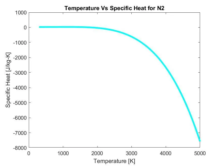
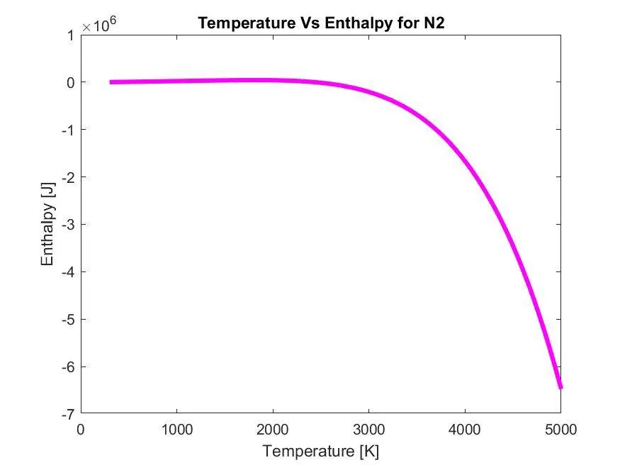
• The plotting command will illustrate the computed data graphically and makes it more visual for interpreting the relationship between the local temperature and thermodynamic properties of the species.
• Prior to plotting the action of creating individual folders becomes inevitable and reason being plots for 53 species becomes difficult to find. ‘mkdir’ and ‘cd’ commands are used to define the working directory in which species specific folders are created to save the plots. To make the plot clear and readable they are labelled and marked where necessary and finally using ‘saveas’ command they are stored in the folder created in the specified format.
• The last bit of the operation involves calculating the molecular weight. This is included as soon the plots are completed, once the value is computed to make it readily available ‘fopen’ command is used to write a file and store the same in ‘.txt’ format in the same folder.
• Final operation involves the ‘fclose’ which will terminate the process after the iterations runs its course.
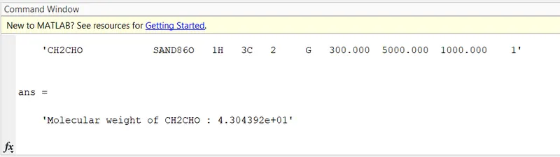
• The molecular weights are also read out in the command window as shown in the pictures attached below. Plots for o2,Co2,N2 are attached for perusal.

Plots and Results:

1. Folders created in the designated working directory:

2. Plots of O2

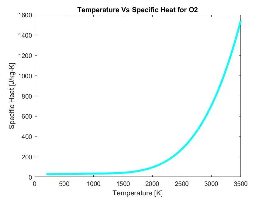
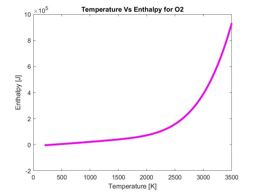
3. Plots for CO2

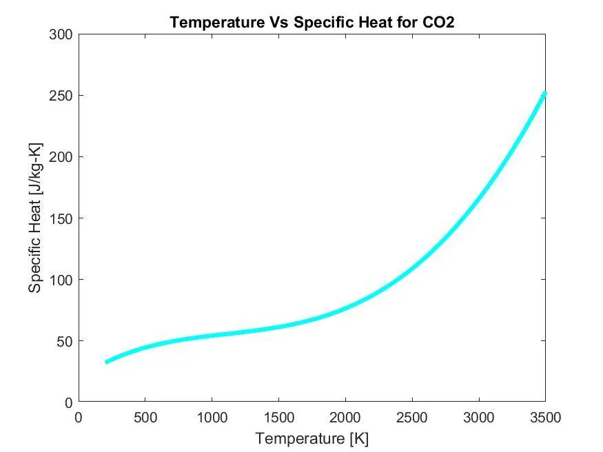
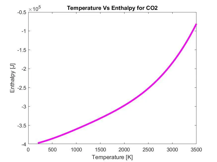
4. Plots for N2

5. Molecular weight Readout in Command Window:

Inference:

In this exercise the 'THERMO.dat' file was parsed and necessary values were extracted to usable formate to compute specific heat, enthalpy, entropy for various species.