Stalagmite Function Optimization in MATLAB

Aim:

Optimize the stalagmite function using the genetic algorithm ‘ga’ command/tool and subsequently find its global maximum’.

Literature Review:

Firstly optimization refers to the process of taking inputs to which best outputs are to be obtained and by definition it refers to minimizing or maximizing object function/s. Here, the set of inputs are populating a search space and through optimization we can locate the optimal point/s.

The Stalagmite Function: [1]

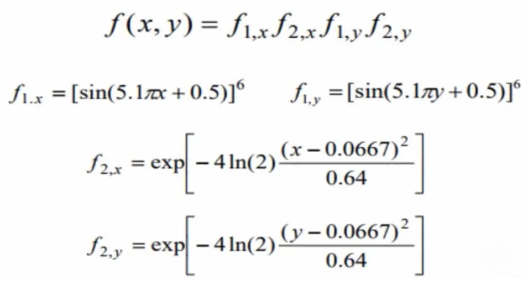
Also one must know that an objective function is being optimized, additionally the fitness function guides this optimization and finally these results are scaled as positive fitness values are required from which best individuals are selected. The fitness value is calculated repeatedly in ‘ga’ and computation of these values can slow down the process.

Insight: Most scenarios the fitness function is nothing but the objective function and the reason is we are trying to minimize or maximize the objective function. However, for cases with multiple objectives and boundaries, it might become necessary to employ different fitness functions. [2].

Understanding the Genetic Algorithm: [2] [3]

1. For an initial randomized population set the algorithm creates new population. Firstly, it uses the initial individuals for current generation for the next generation to come.
2. For initial individuals the fitness value is computed and used to score them in the group. These fitness values are scaled for selecting the members, over here the scaled values are called expectation.
3. The members selected above for procreation are termed as parents. However, there are a group of parents selected based on best fitness values and passed on to the next population.
4. These parents produce children:

• First kind are produced by combining the vector entries of the parents, called crossover
• Second kind are produced from single parent by making random changes, called mutation

5. The algorithm replaces the above as next generation. Since, this process can be done endlessly, one must initiate a stopping point.
6. The ‘ga’ tool comes with the stopping condition option viz., ‘optimoptions’ in which the below mentioned conditions can be applied

• ‘MaxGeneration’ – stops when it reaches the specified maximum generation value
• ‘FitnessLimit’ – when the value of the fitness function for the initial population is less than or equal to the ‘FitnessLimit’ it will stop.
• ‘MaxTime’ – a timer can be set that will end terminate the algorithm

In Darwin’s ‘Theory of Evolution’, the section ‘survival of the fittest’ was used as inspiration to device this search based algorithm. For real world problems this algorithm can be translated or understood as: the population or initial generation are considered as solution set for a problem and as explained there is a component of reproduction (crossover and mutation) which is nothing but production of new children. [4]

Reproductions if crossover there exists three types single point crossover that considers one random point on both parents’ chromosomes for crossover. Similarly, there is two-point cross over where two points are considered and finally, uniform crossover where all the chromosomes are chosen with equal probability for crossover. If mutation occurs to avoid convergence of results to happen sooner than intended and create diversity by flipping any bit of the chromosome.

The children solutions yielded will be added to the population for further iterations. Also, the whole process being randomized the user can specific focus region (localize) of the yielded solutions to get a better random local search. [5]

Merits and Demerits:

Unlike any other optimization tools available the ‘ga’ comes with its merits such as: helps in solving multiple objective problems that are prevalent in the real world, provides an array of solutions to choose from and most importantly real time data aren’t derivative which is handled well by ‘ga’. [6]

Merits aside, the very obvious demerits are the solutions produced by ‘ga’ not necessarily converge to optimal solution, computational expense can be more for few problems when the fitness loop is required to run extensively. [6]

‘ga’ syntax Explanation: [7]

x = ga(fun,nvars) – finds a local unconstrained minimum “x”, to the objective function “fun”. The number of design variable of the function are given by “nvars”.

x = ga(fun,nvars,A,b) – finds local minimum “x” but subjected to linear equalities Aeq*x = beq and A*x ≤ b. (make A=[] and b=[] if no linear inequalities exist.) ga evaluates the matrix product Aeq*x as if x is transposed (Aeq*x')

x = ga(fun,nvars,A,b,Aeq,beq,lb,ub) -- here the lower bound “lb and upper bound “ub” are imposed on the design variables “x” to focus solution in the range lb ≤ x ≤ ub. However, if no linear equalities exist then make Aeq=[] and beq=[]

x = ga(fun,nvars,A,b,Aeq,beq,lb,ub,nonlcon) – minimization is constrained by nonlcon and this function accepts x and returns two vectors C and Ceq, which is non-linear inequalities an equalities respectively. ‘ga’, then minimizes the function such that C(x) ≤ 0 and Ceq(x) = 0

x = ga(fun,nvars,A,b,Aeq,beq,lb,ub,nonlcon,options*) using optimoptions [8] command create options and the values in the options replaces the optimization parameters shown below

[8]

x = ga(problem) -- finds the minimum for structure described in problem.

[x,fval] = ga(___) -- it also returns the value of the fitness function at x.

[x,fval,exitflag,output] = ga(___) also returns exitflag that identifies the reason for termination along with output which contains performance and outputs of each generation

[x,fval,exitflag,output,population,scores] = ga(___) – in addition here it returns final population and its vector scores

Matlab code:

Stalgamite function:

function f = stalagmite(input_vector)

        fx1 = (sin(5.1*pi*input_vector(1) + 0.5))^6;  % first equation as seen in the stalagmite function
        fy1 = (sin(5.1*pi*input_vector(2) + 0.5))^6;  % second equation as seen in the stalagmite function
    
            k1 = ((input_vector(1)-0.0667).^2)/(0.64);
            fx2 = exp(-4.*log(2)*k1);                 % third equation as seen in the stalagmite function
            k2 = ((input_vector(2)-0.0667).^2)/(0.64);
            fy2 = exp(-4.*log(2)*k2);                 % fourth equation as seen in the stalagmite function
    
    f = -(fx1.*fx2.*fy1.*fy2);   % final equation in the stalagmite equation 

end

Plotting Stalagmite function:

Code:

% Clear workspace
clear all
close all
clc

% creating search space 
x = linspace(0,0.6,150);
y = linspace(0,0.6,150);

% ga will iterate to evaluate the fitness 
n = 50; 

% create meshgrid in 2D for the interations  
[xx, yy] = meshgrid(x,y);

% To evaluate Stalagmite function

tic 
for i = 1:length(xx)
        for j = 1:length(yy)
            input_vector(1)=xx(i,j);
            input_vector(2)=yy(i,j);
            f(i,j) = stalagmite(input_vector);
        end
        
end
 study_time = toc; % tic & toc command is used to record the total time for deriving the results
 
% to plot stalagmite function 
 surfc(xx,yy,-f) 
shading interp
xlabel('x-value')
ylabel('y-value')
zlabel('function value')
title('Stalagmite function')

Plot:

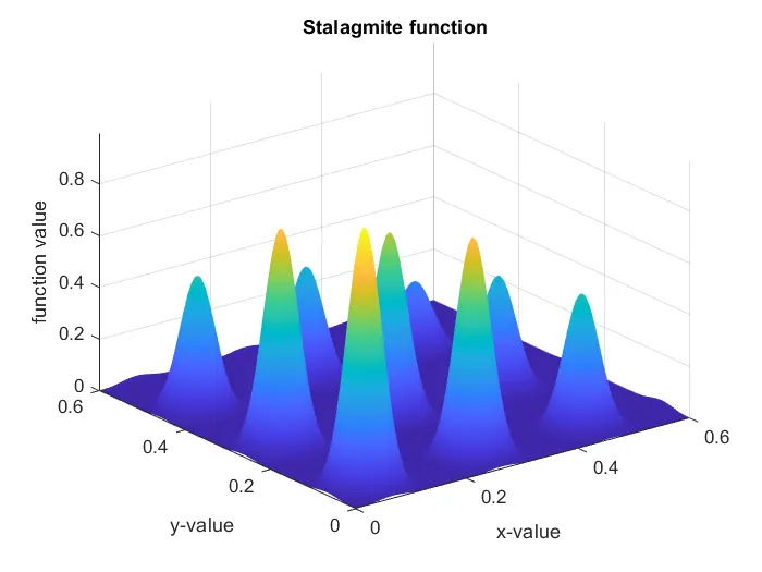
Study #1: Studying the statistical behaviour of Unbounded inputs

MATLAB code:

% Clear workspace
clear all
close all
clc

% search space 
x = linspace(0,0.6,150);
y = linspace(0,0.6,150);

% ga will iterate to evaluate the fitness
n_iterations = 50; 

% create meshgrid in 2D   
[xx, yy] = meshgrid(x,y);

% Stalagmite function evaluation for surface plot 

for i = 1:length(xx)
        for j = 1:length(yy)
            input_vector(1)=xx(i,j);
            input_vector(2)=yy(i,j);
            f(i,j) = stalagmite(input_vector);
        end
        
end

% To Plot Unbounded Statistical approach

tic % starts the stopwatch 
for i=1:n_iterations
[inputs1,fopt1(i)]=ga(@stalagmite,2);
xopt1(i)=inputs1(1);
yopt1(i)=inputs1(2);
end

% surface and 
study1_time=toc; % records the time taken for the iterations
% to plot the statistical behaviour of the unbounded inputs 
figure(1)
subplot(2,1,1) 
surfc(xx,yy,-f)
shading interp
hold on
xlabel('x-value')
ylabel('y-value')
zlabel('function value')
plot3(xopt1,yopt1,-fopt1,'marker','o','markersize',5,'markerfacecolor','r')
title('Unbounded')
hold on

subplot(2,1,2)
plot(-fopt1)
xlabel('iterations')
ylabel('function maximum')

Results:

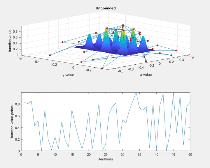
Looking at the above plot the results are unclear and cannot be used in real time.

Study #2: Studying the statistical behaviour of bounded inputs

In this approach the lower and upper bounds are defined which leads to confined boundation of the results.

MATLAB Code:

% Clear workspace for studying statistical behaviour of bounded inputs
clear all
close all
clc

% create search space
x = linspace(0,0.6,150);
y = linspace(0,0.6,150);

% ga iterations to evaluate fitness 
n = 50; 

% create meshgrid in 2D for the interations  
[xx, yy] = meshgrid(x,y);

% to evaluate the Stalagmite function

for i = 1:length(xx)
        for j = 1:length(yy)
            input_vector(1)=xx(i,j);
            input_vector(2)=yy(i,j);
            f(i,j) = stalagmite(input_vector);
        end
        
end

% to evaluate statistical behaviour of bounded inputs 
tic
for i=1:n
[inputs1,fopt2(i)]=ga(@stalagmite,2,[],[],[],[],[0;0],[0.6;0.6]);
xopt(i)=inputs1(1);
yopt(i)=inputs1(2);
end
study2_time=toc; % tic & toc command is used to record the total time for deriving the results

% to plot and understand the statistical behaviour of bounded inputs
figure(1)
subplot(2,1,1) 
surfc(xx,yy,-f)
shading interp
hold on
xlabel('x-value')
ylabel('y-value')
zlabel('function value')
plot3(xopt,yopt,-fopt2,'marker','o','markersize',5,'markerfacecolor','r')
title('Bounded statistical Behaviour')
hold on

subplot(2,1,2)
plot(-fopt2)
xlabel('iterations')
ylabel('function value points')

Results:

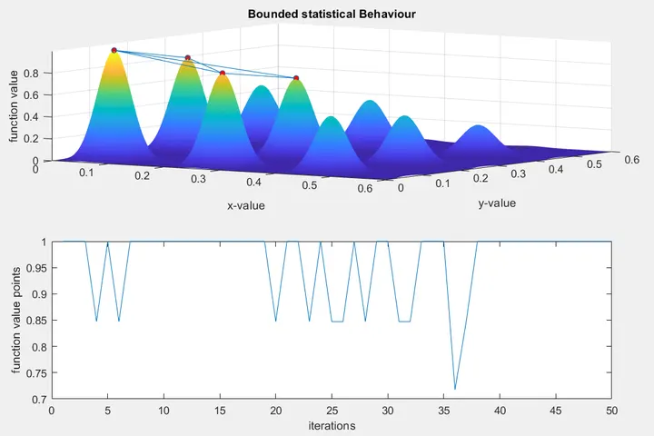
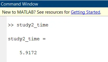
Eventhough the results seems to much more refined these need to be further investigated and made better and the next study is does the same.

study time recorded :

Study #3: Studying the statistical behaviour of bounded inputs by modifying population size

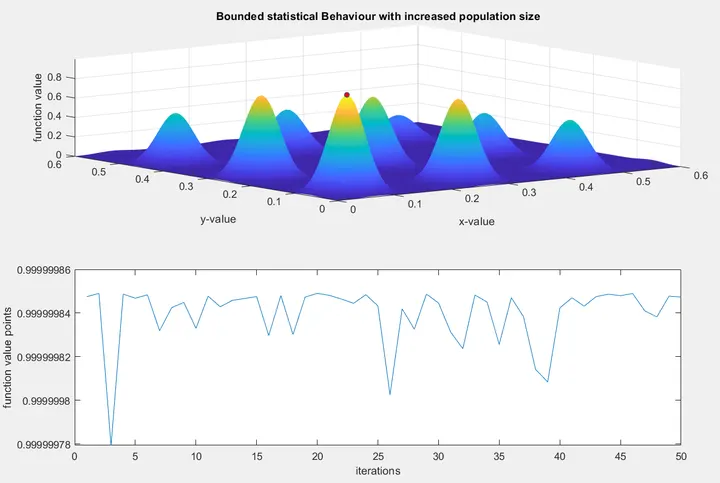
By doing so we can find the global maxima instead of local maxima which was seen in the earlier study.

MATLAB Code:

% Clear workspace to study the statistical behaviour of bounded inputs with
% modified population size
clear all
close all
clc
x = linspace(0,0.6,150);
y = linspace(0,0.6,150);
% ga will iterate to evaluate the fitness 
n = 50; 
% create meshgrid in 2D for the interations  
[xx, yy] = meshgrid(x,y);
% Stalagmite function
for i = 1:length(xx)
        for j = 1:length(yy)
            input_vector(1)=xx(i,j);
            input_vector(2)=yy(i,j);
            f(i,j) = stalagmite(input_vector);
        end
        
end
% population size increase using optimoptions command for including options
% in ga as seen below 
% default population size considered is 50
options = optimoptions(@ga,'populationsize',300); 
% to evaluate statistical behaviour for bounded with modified population size 
tic
for i=1:n
[inputs1,fopt3(i)]=ga(@stalagmite,2,[],[],[],[],[0;0],[0.6;0.6],[],[],options);
xopt(i)=inputs1(1);
yopt(i)=inputs1(2);
end
study3_time=toc; % tic & toc command is used to record the total time for deriving the results

figure(1)
subplot(2,1,1)
 
surfc(xx,yy,-f)
shading interp
hold on
xlabel('x-value')
ylabel('y-value')
zlabel('function value')
plot3(xopt,yopt,-fopt3,'marker','o','markersize',5,'markerfacecolor','r')
title('Bounded statistical Behaviour with increased population size')
hold on
%figure(2)
subplot(2,1,2)
plot(-fopt3)
xlabel('iterations')
ylabel('function value points')

Results:

study time recorded :

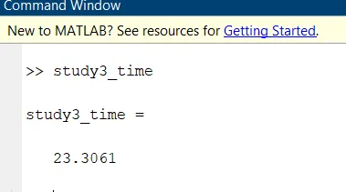
It can be observed that the time taken for computation significantly increased, however the results tends to converge and seem much better than the first two studies.

Conclusion:

Further to this, one can change the number of iterations and population size in order to get better results and this at the cost of compting time. This study gives a rudimentary understanding on how the Genetic Algorithm functions and how it can be applied for optimizing problems.

References

[1]	Skill-Lync, "Genetic Algorithm Explained," [Online]. Available: https://skill-lync.freshdesk.com/support/solutions/articles/43000584189-genetic-algorithm-explained-#:~:text=Genetic%20Algorithm%20(GA)%20is%20a,optimal%20or%20near%2Doptimal%20solutions..
[2]	T. Point, "Genetic Algorithms - Fitness Function," [Online]. Available: https://www.tutorialspoint.com/genetic_algorithms/genetic_algorithms_fitness_function.htm.
[3]	MathWorks, "How the Genetic Algorithm Works," MathWorks, [Online]. Available: https://in.mathworks.com/help/gads/how-the-genetic-algorithm-works.html#f6243.
[4]	T. Back, "Biological Background," in Evolutionary Algorithms in Theory and Practice.
[5]	T. Back, "Evolutionary Alogorithms and Global Optimization," in Evolutionary Algorithms in Theory and Practice, New York, Oxford Press, 1996, pp. 34-62.
[6]	MathWorks, "Genetic Algorithm - Find global minima for highly non-linear problems," MathWorks, [Online]. Available: https://in.mathworks.com/discovery/genetic-algorithm.html.
[7]	MathWorks, "ga," MathWorks, [Online]. Available: https://in.mathworks.com/help/gads/ga.html.
[8]	MathWorks, "optimoptions," MathWorks, [Online]. Available: https://in.mathworks.com/help/optim/ug/optim.problemdef.optimizationproblem.optimoptions.html#btm45w6-2.