Week 3 - Solving second order ODEs

Pendulum Problem

Aim: To simulate / trace the motion of the pendulum bob using the second order equation that describes its motion.

Code:

The equation being second order needs to be converted into two ordinary differential equations that can be utilised for the time based iterations. Alternatively, the simple pendulum can be viewed as a system of spring-mass-damper and equation below gives the idea of the system in motion.

Steps incorporated to split the above equation into two first order differential equation;

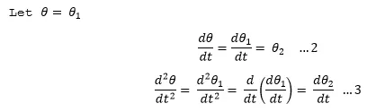
Then the original equation ‘1’ can be written as;

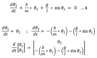
The above equation is the converted into function and ode45 solver is used for computing the displacement and angular velocity. This function is named as ode_func and is integrated over the time span of ‘0 to 20 seconds’. The same notations used in deriving the above equations are used in the ode_func below;

function [dtheta_dt] = ode_func(t,theta,b,g,l,m)

theta1 = theta(1);
theta2 = theta(2);
dtheta1_dt = theta2;
dtheta2_dt = -(b/m)*theta2 - (g/l)*sin(theta1);
dtheta_dt = [dtheta1_dt; dtheta2_dt];
end
 

In continuation the above function is called in the below mentioned program, and the same is plotted for every instance. This captured data is stored in the form of frames with the use of ‘getframe’ command and the loop counter ‘ct’ is used for every successive iteration to be run and ‘VideoWriter’ stitches all the frames together and stores it in the .avi format. The ‘Marker’ and ‘Markersize’ is used for the pointers that trace the path on the graph as well as for the pendulum bob.

The ‘sprintf’ command is employed to see the time steps at which the animation and the plots are getting traced. Lastly, the fprintf is a command that is used to format as well as display the ‘tic’ and ‘toc’ commands used for the animation. The constants used ie.,

b = damping coefficient, m = mass, l = length of the pendulum, the initialisation of the time step at time 't0' the angular velocity is 3rads/sec and the acceleration due to gravity = g are all mentioned in the code with explation beside them.

% Clear the workspace 
clear all
close all
clc

% Pendulum parameters - constant 
b = 0.05;    % Damping co-efficient
m = 1;       % Mass of the pendulum bob  [kg]
g = 9.81;    % Acceleration due to gravitational [m/s^2]
l = 1;       % Length of the pendulum [m]

% Initialising the problem angular displacement=0 & angular velocity is 3
% 3 rad/ sec at time t=0 seconds 
theta_0 = [0;3]; 

% time span for which the problem is integrated
t_span = linspace(0,20,500);

%solve the second ode using ode_func
[t, results] = ode45(@(t,theta) ode_func(t,theta,b,g,l,m), t_span, theta_0);

% To plot the pendulum location for iteration 
       x = l*sin(results(:,1));
       y = -l*cos(results(:,1));

% radians converted to angles that are needed for simulating the pendulum       
% angle = results(:,1:2)*180/pi; in case we define in deg 

% To simulate the plot in accordance to the actual pendulum movement
figure(1)
subplot(2,1,1);

% Loop counter for the iterations 
ct = 1;

tic;
for i = 1 : length(t)
    % The line plot that represents the function and the marker traces the
    % simulation of the pendulum bob at every time step
    subplot(2,1,1);       
    plot(t,results,'LineWidth',2);
    line(t(i), results(i,1),'Marker','.','MarkerSize',20,'Color','b');
    line(t(i), results(i,2),'Marker','.','MarkerSize',20,'Color',[0 .5 0]);
   
    % legend('Displacement [rad]','Angular Velocity [rad/sec]') mentioning
    % this on a legend makes the set up combersome and has been avoided
    
    % Angular Velocity [rad/sec],Displcament [rad]
    xlabel('time [s]'); ylabel('Ang Vel[rad/s] & Disp');
    
       % The animation of the pendulum for the given paramters
       subplot(2,1,2);
       plot([0,x(i,1)],[0,y(i,1)],'.-','MarkerSize',20,'Color','k','LineWidth',2); % the pendulum and the bob is colored black
       hold on
       plot([-0.5 0.5],[0 0],'LineWidth',5,'Color','y'); % anchoring point of the pendulum is yellow 
       axis equal; axis([-2*l 2*l -2*l 2*l]);
       title(sprintf('Time: %0.2f sec',t(i)));
    
    % Updating figures for process
    drawnow;
    % To capture all the iterations in frames
    M(ct) = getframe(gcf);
    hold off 
    ct = ct + 1;
end

% to format data and display the results'Angular Velocity [rad/sec]
fprintf('Animation(Regular): %0.2f sec\n',toc);
 
% using the movie command to compile all the frames
 movie(M)
 % video writer command to get .avi format video file 
 vid = VideoWriter('Pendulum_Animation.avi','Uncompressed AVI');
 open(vid)
 writeVideo(vid,M)
 close(vid)

Troubleshooting and solving them:

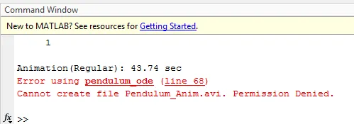
1. The animation was created and when the code was executed once again after a few minor changes the video was not over written and the file Pendulum_Anim.avi had to be changed to Pendulul_Animation.avi in order to solve this issue.

2. Array used to plot all the position of the pendulum bob was chosen as results and this was avoided by using the i itself that was the entire length of values from the results for the said time step.

Inference: Please follow the below link for the animation

https://youtu.be/gCVDvp7Pg_w