Week 3 - Solving second order ODEs

AIM- To write a program that solves the following ODE which represents the equation of motion of a simple pendulum with damping and simulate the motion between 0-20 sec, for angular displacement=0, angular velocity=3 rad/sec at time t=0. When you do this you will get the position of the pendulum as a function of time. Use this information to animate the motion of the pendulum, as shown in the below figure.

INTRODUCTION- An ordinary differential equation is an equation that involves some ordinary derivatives (as opposed to partial derivatives) of a function. Often, our goal is to solve this ordinary differential equation i.e., determine what function or functions satisfy the equation.

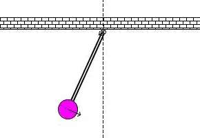
Animation of pendulum

In mathematics, the term “Ordinary Differential Equations” is an equation that contains only one independent variable and one or more of its derivatives with respect to the variable. In other words, the ODE is represented as the relation having one independent variable x, the real dependent variable y, with some of its derivatives.

In Engineering, it is used to describe the transient behavior of a system. This is extremely important in engineering, as it is used to describe lot of important phenomena and solving this equation may help to understand the system in real life. Some of the example are pendulum, spring, damper and mass system. The way the pendulum moves depends on the Newtons second law. When this law is written down, we get a second order Ordinary Differential Equation that describes the position of the "ball" w.r.t time. It is abbreviated as ODE.

Similarly, there are hundreds of ODEs that describe key phenomena and if you have the ability to solve these equations then you will be able to simulate any of these systems. An ODE usually represents the equation of motion of a simple pendulum with damping. An ordinary differential equation is an equation which is defined for one or more functions of one independent variable and its derivatives. y'=x+1 is an example of ODE.

Application- ODEs has remarkable applications and it has the ability to predict the world around us. It is used in a variety of disciplines like biology, economics, physics, chemistry and engineering. It helps to predict the exponential growth and decay, population and species growth. Some of the uses of ODEs are:

• Modelling the growth of diseases
• Describes the movement of electricity
• Describes the motion of the pendulum, waves
• Used in Newton’s second law of motion and Law of cooling

Main Objectives-

• For each value of time, create an image that represents the position of the pendulum.
• Assume the length of the string and the size of the ball.
• Use the marker command to create a sphere.
• One end of the pendulum is fixed.
• The other end moves according to the solution of the ODE that you had solved.
• If you are using Matlab, use the movie command to create an animation.

A second order differential equation cannot be solved directly in matlab, in order to solve this second order differential equation it needs to be converted into first order differential equation. Here, one second order differential equation can be converted into two first order equations. Fundamental idea behind behind solving this ODEs is both analytically andcomputationally as when you have higher ODE, then you have to break it down to a set of first order ODE.

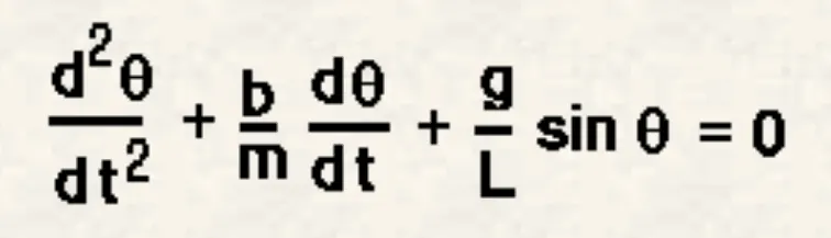------------------------>(1)

where, g=acc due to gravity (in m/s^2) L=length of pendulum (in m) m=mass of ball (in kg) b = damping coefficient

Value and parameters to be used to solve the above equation of the pendulum

L=1 metre,

m=1 kg

b=0.05.

g=9.81 m/s^2.

A Second-order equation cannot be solved directly solved in the Matlab, in order to solve a second order equation it needs to be converted into First order equation. One second order equation can be converted into two first-order equations.

Below are the two first-order equations which are calculated by splitting a second order equation that equation (1).

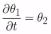--------------->(2)

From this above equation (EQUATION 1) is derieved to be

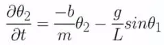---------------->(3)

Equation (2) and (3) are the two first order differential equations which is calculated by splitting a second order equation from equation(1).

Upon calculating the first equation, angular velocity can be determined and by calculating the second equation, angular acceleration can be determinded.

Main Program

%Clearing the screen, command line, Work space and closing all plots
clear all
close all
clc

%Initial Conditions
theta_0 =[0;3];

%Time
t_span=linspace(0,20,600);

[t,results]=ode45(@ode_pendulum_damped_func,t_span,theta_0);

figure(1)
subplot(1,2,1)
plot(t,results(:,1),'color','b')
xlabel('Time')
ylabel('Angular velocity')
title('Variation of angular displacement with respect to time')
subplot(1,2,2)
plot(t,results(:,2),'color','r')
xlabel('Time')
ylabel('Angular velocity')
title('Variation of angular velocity with respect to time')

figure(2)
plot(t,results(:,1),'color','b')
hold on
plot(t,results(:,2),'color','r')
xlabel('Time')
ylabel('Angular displacement and angular velocity')
legend('Angular displacement','Angular velocity')
title('Variation of angular displacement over angular velocity with respect to time')
disp=results(:,1);
ct=1;

for i=1:length(disp)
    THETA=disp(i);
    l=1;
    x0=0;
    y0=0;
    x1=l*sind(THETA);
    y1=-l*cosd(THETA);
    figure(3)
    plot([1 -1],[0 0],'linewidth',6,'color','g')
    hold on
    plot([x0,x1],[y0,y1],'linewidth',3,'color','r')
    axis([-1 1 -1 0])
    hold on
    plot(x1,y1,'O','markers',30,'markerfacecolor','b')
    hold off
    pause(0.001)
    
    M(ct)=getframe(gcf);
    ct=ct+1;
end

%Creating the animation for damped pendulum
 %Inserting frames in the animation to make a movie(.avi) 
 movie(M)
 videofile=VideoWriter('Pendulum_damped.avi','uncompressed AVI');
 open(videofile)
 writeVideo(videofile,M)
 close(videofile)

Function Program

%function to run ode_pendulum_damped code
function[dtheta_dt]=ode_pendulum_damped_func(t,theta)
 %Inputs
 l = 1;   %(in m)
 m = 1;   %(in kg)
 b = 0.05;
 g = 9.8; %(in m/s^2)
 t=-(b/m)*theta(2)-(g/l)*sin(theta(1));
 dtheta_dt = [theta(2);t];
end

Stepwise Explanation for the first program and function code:

1. In the first step has a regular Practise started the program with clear all, close all and clc commands which will help in clearing temporary memory, closing current plots which are opened and clearing the command prompt respectively.

2. Next array of time is generated by using the command linspace. t_span=linspace(0,20,500). Here this command creates 600 time slots in the range of 0-20 sec.

3. Next initial conditions for angular displacement and angular velocity have defined has 0 and 3 respectively.

4. In the next line ode45 function has defined which is assigned to the array [t, results].Here in the above array results again has 2 columns in which column 1 defines angular displacement and column 2 defines angular velocity.

5. Once execution reaches to ode45 function the which is defined as ode45(@ode_pendulum_damped_func,t_span,theta_0) which has another function ode_pendulum_damped_func will be called and then by using initial conditions MATLAB integrates time and with respect to that result, an array will be calculated. ode_pendulum_damped_func has the function which calculates two first-order equations of simple pendulum equation.

6. Now once after generating the result array which has 2 columns one has displacement and other has velocities by utilising these values individual plots are generated. Here 2 plots are generated which are in turn shown under a single figure by using subplot command.

plot1: It shows Variation of angular displacement with respect to time.

subplot(1,2,1)
plot(t,results(:,1),'color','b')
xlabel('Time')
ylabel('Angular displacement')
title('Variation of angular displacement with respect to time ')

In the above code, the subplot command is used to show different plots in a single figure.

plot2: It shows Variation of angular velocity with respect to time

subplot(1,2,2)
plot(t,results(:,2),'color','r')
xlabel('Time')
ylabel('Angular velocity')
title('Variation of angular velocity with respect to time ')

7. Now in the figure(2), it is shown how angular displacement and angular velocity changes with respect to time.

8. Now once after generating angular displacement value with respect to this angular displacement values simple pendulum need to generate having length 1m and mass 1 kg.

9. 1 column of the results is assigned to a variable called displacement and ct=1 has been defined in order to initiate the loop and in the for loop simple pendulum with respect to theta is defined as

x0=0;
y0=0;
x1=l*sind(THETA);
y1=-l*cosd(THETA);

where THETA is an angular displacement with respect to the value of i. After plot command, the new axis dimension have been allotted using the command

axis([-1 1 -1 0]), here x axis is dimensioned with starting limit -1and last limit 1,

y axis is dimensioned with starting limit -1 and last limit 0.

10. Now figure(3) is plotted which consists of plotting of simple pendulum rod and ball. A ball is generated by using command plot(x1,y1,'o','markers',30,'markerfacecolor','b').

pause(0.001) is used to slow down the animation for every combination of theta by 0.001, which helps easy understanding of animation pause(0.001)

11. capturing the frame for every value of counter getframe command is used and obtained frame is assigned to M and after the value of a counter is incremented by M(ct)=getframe(gcf); ct=ct+1;

12. After above for loop a movie is generated using the function movie which has the frame obtained by using M. movie(M)

13. Now creating the video file of avi format using vediowriter function having ode_pendulum_task.avi as the file name which is an uncompressed avi file videofile=VideoWriter('ode_pendulum_task.avi','uncompressed AVI')

14. Once vediofile is created that particular file is opened by using open function and by using writeVedio function particular video file is written by using Frames of M and then once all the frames are written file is closed using close function. open(videofile) writeVideo(videofile,M) close(videofile)

RESULTS

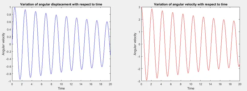
Figure 1: Variation of angular displacement with respect to time and variation of angular velocity with respect to time

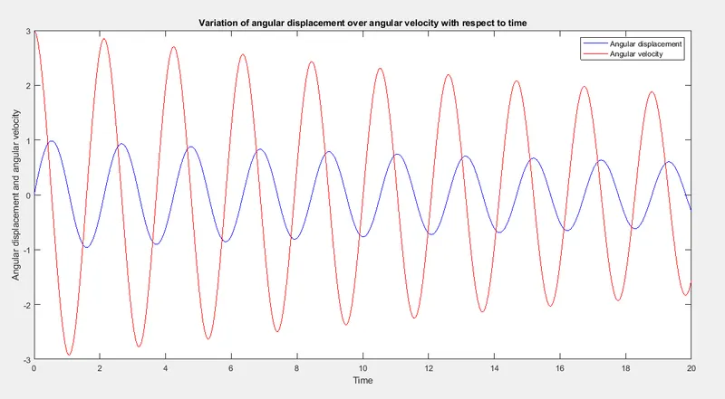
Figure 2: Variation of angular displacement over angular velocity with respect to time

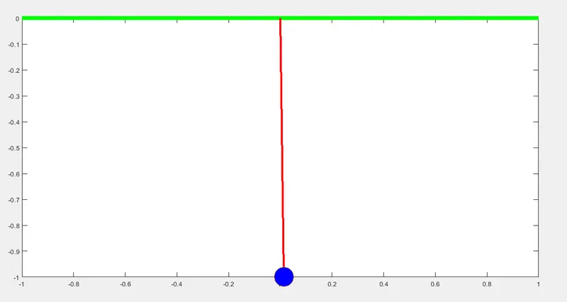
Figure 3: An image of the animation of the Damped pendulum

Animation of Simple Damped Pendulum:- https://youtu.be/s59I7iuBJ1Y