Week 3 - Solving second order ODEs

Aim:

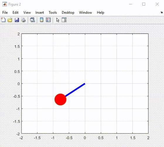
To write a program that solves the following Second ODE. This ODE represents the equation of motion of a simple pendulum with damping and creating an animation.

Objective:

The second-order differential equation of motion of simple pendulum with damping is

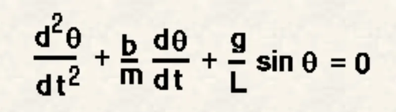
where

g = gravity in m/s2,

L = length of the pendulum in m,

m = mass of the ball in kg,

b=damping coefficient.

Given inputs

L=1 metre,

m=1 kg,

b=0.05.

g=9.81 m/s2.

Simulate the motion between 0-20 sec, for angular displacement=0,angular velocity=3 rad/sec at time t=0.

Theory:

Ordinary Differential Equations:
In mathematics, an ordinary differential equation (ODE) is a differential equation containing one or more functions of an independent variable and the derivatives of those functions. The term ordinary is used in contrast with the term partial differential equation which maybe for more than one independent variable.

Simple Pendulum:
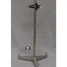
A pendulum is a body suspended from a fixed support so that it swings freely back and forth under the influence of gravity. When a pendulum is displaced sideways from its resting, equilibrium position, it is subject to a restoring force due to gravity that accelerates it back toward the equilibrium position. When released, the restoring force acting on the pendulum's mass causes it to oscillate about the equilibrium position, swinging it back and forth. The mathematics of pendulums are in general quite complicated. Simplifying assumptions can be made, which in the case of a simple pendulum allow the equations of motion to be solved analytically for small-angle oscillations.

Working Principle:
In mechanics and physics, simple harmonic motion is a special type of periodic motion or oscillation where the restoring force is directly proportional to the displacement and acts in the direction opposite to that of displacement. The best example of the simple Harmonic motion is a Simple Pendulum motion.

A pendulum consists of a massless rod, a Frictionless pivot, a bob. The simple gravity pendulum is an idealized mathematical model of a pendulum. This is a weight (or bob) on the end of a massless cord suspended from a pivot, without friction. When given an initial push, it will swing back and forth at a constant amplitude. Real pendulums are subject to friction and air drag, so the amplitude of their swings declines. The pendulum works on Newton Second Law and a Second Order Ordinary Differential Equations (ODE) are formed that describe the position of the pendulum concerning time.

Equation Used:

The second-order ODE for a simple pendulum

[`d^2``theta``dt^2`]+[(b/m )(d`theta`/dt)]+(g/L)sin`theta`=0 .....(1)

To change the ODE from `2^nd` order to `1^st` order,

let

`theta`= `theta1`

therefore, Equation(1) becomes

``[d`theta`/dt]` = `[d`theta1`/dt]` =theta2`.......(2)

`d^2``theta`/`dt^2` = `d^2``theta1`/`dt^2` = d/dt(d`theta1`/dt) = d`theta2`/dt .........(3)

Substitute Eqn (2) and (3) in Equation (1)

Therefore the Equation becomes

[`d^2``theta1`/`dt^2`]+[(b/m )(d`theta1`/dt)]+(g/L)sin`theta1`=0

[d`theta2`/dt]+[(b/m )(`theta2`)+(g/L)sin`theta1`=0

[d`theta2`/dt] = -[(b/m )(`theta2`)-(g/L)sin`theta1`

To arrange it in the matrix form

d`theta`/dt = d/dt(`theta1`,`theta2`) = (`theta2`, -b/m`theta2`-g/Lsin`theta1`)

Main Code:

clear all
close all
clc

% Inputs
b = 0.05; % co-eff of damping
g = 9.81; % {metre/second^2}
l = 1; % {lenght in metre}
m = 1; % {mass in kilograms}

% Initial Condition
theta_0 = [0;3];

% Time Points
t_span = linspace(0,10,100);

%Solve ODE
[t,results] = ode45(@(t,theta)ode_func(theta,b,g,l,m),t_span,theta_0);

figure(1)
plot (t,results(:,1))
hold on
plot (t, results(:,2))
ylabel('amplitute')
xlabel('time')
grid on

legend(['displacement(rad)','Velocity[rad/sec)'])
hold off
ct=1;

for i=1:length(t_span)
    theta = results(:,1)
    angular_velocity = results(:,2);
    x0 = 0;
    y0 = 0;
    x = l*sin(theta(i));
    y = -l*cos(theta(i));
    
    %ploting
    figure(2)
    
    plot(0,0,'o','Markersize',30,'color','b','Markerfacecolor','g')
    plot([0,x],[0,y],'linewidth',4,'color','b')
    hold on
    plot(x,y,'-o','markers',30,'markerfacecolor','r')
    axis([-2 2 -2 2])
    hold off
    grid on 
     
    %collecting frame of figures to create animation
    M(ct) = getframe(gcf);
 
    ct = ct+1;
end
movie(M)
videofile = VideoWriter('pendulum_ODE.avi','uncompressed AVI');
open(videofile)
writeVideo(videofile,M)
close(videofile)

Explanation:

The fixed parameters are length, mass, damping coefficient, and acceleration due to gravity in the above program.
Time and angle are given as the initial condition.
In the t-span command, 100 values are taken in between 0 to 10 times period.
Using the ode 45 command ODE function is introduced.
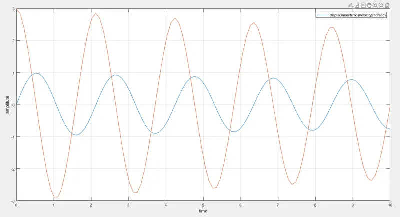
Using the plot command velocity and displacement are plotted in the y-axis against time in the x-axis.
Using the for loop command, the mass at various points and various times are marked in the graph and plotted.
Using the movie command the plot is saved as uncompressed. AVI file.

Function Code:

function [dtheta_dt] = ode_func(theta,b,g,l,m)

theta1 = theta(1)
theta2 = theta(2)
dtheta1_dt = theta2;
dtheta2_dt = -(b/m)*theta2-(g/l)*sin(theta1);
dtheta_dt = [dtheta1_dt;dtheta2_dt];
end

Explanation:
In this function program, the second-order ODE is simplified to the first-order ODE by introducing the term theta1 & theta2
Then theta1 & theta2 are differentiated and the dtheta_dt gives a column matrix.

GRAPH:

Amplitude vs Time:

Animation: