Week 3 - Solving second order ODEs

AIM: To write a program for simulating the transient behaviour of a simple pendulam.

OBJECTIVES:

• Solve the second order ODE for the motion of a simple pendulam.
• Generate a plot for its angular displacement and angular velocity w.r..t time.
• Create an animation for the motion of the pendulam.

GOVERNING EQUATIONS:

Ordinary differential equation for oscillating motion of non linear pendulam is

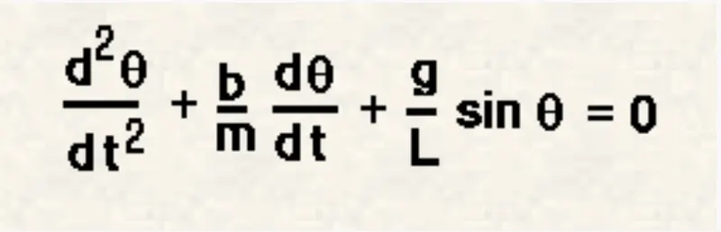
here,

g= gravity in(m/s^2)

l= length of the pendulam in (m)

m= mass of the ball in (kg)

b= damping coefficient

INPUT VARIABLES:

The input variables which are required for the programming is as follows-

l=1m

m=1kg

b=0.05

g=9.81m/s^2

THEORY:

In Mathematics an ordinary differentian equation is a differential equation containing one or more functions of one independent variable and the derivatives of those functions.

ODE is used to derive the transient behaviour of a system. A simple pendulam is the basic example of the ODE. The way pendulam moves is in accordance to the Newtons law of motion and when it is written down in the mathematical formula we get the second order differential equation that describes the position of ball w.r.t time.

The above equation shows us the 2nd order differential equation of simple pendulam with damping.

A pendulum is a weight suspended from a pivot so that it can swing freely. When a pendulum is displaced sideways from its resting, equilibrium position, it is subject to a restoring force due to gravity that will accelerate it back towards the equilibrium position. When released the restoring force acting on pendulums mass causes it to oscillate about equilibrium position, swinging back and forth.

STEPS:

In starting we will add our basic libraries which are essential for the solving of the second order ODE which are "math","matplotlib","numpy",and at last the "odeint" from the "scipy" module. This odeint is very essential for solving any ODE in the python.

To start with programming we will first define our function named as "ode_funtion" which is helpful in storing some data like our input variables time span etc.

The given ODE is solved by first converting it into two single order odes for the ease calculation. We will solve it by using the ODEINT command followed by proper syntax and calling the function. These results will plot our angylar displacement and the angular velocity which we get after the calculation with respect to time.

After that we will create the animation of the obtained results for the motion of the pendulam for that FOR loop is used and counter value is initiated,. In this one end is fixed and other end moves according to the solution vector of ODE and is plotted for each time interval of our time span and then we will save our figures according to the loop sp that we can create animation of it in last.

# A program to solve Second Order ODE


import math
import matplotlib.pyplot as plt
import numpy as np
from scipy.integrate import odeint 


#Function that returns dtheta/dt

def ode_function(theta,t,b,g,l,m):
	theta1=theta[0]
	theta2=theta[1]
	dtheta1_dt=theta2
	dtheta2_dt=-(b/m)*theta2-(g/l)*math.sin(theta1)

	dtheta_dt=[dtheta1_dt,dtheta2_dt]
	return dtheta_dt

#Input variables
b=0.05    #Damping coefficient
g=9.81    #Gravity
l=1       # Length of pendulam
m=1       #Mass of bob

#Initial Conditions
theta_0=[0,3]

#Time points
t=np.linspace(0,20,150)

#Solving ODE
theta=odeint(ode_function,theta_0,t,args=(b,g,l,m))

#plotting the graph
plt.plot(t,theta[:,0],'b-',label=r'Angular Displacement(rad)')
plt.plot(t,theta[:,1],'r--',label=r'Angular Velocity(m/s^2)')
plt.xlabel('Time(sec)')
plt.ylabel('Plot')
plt.title('Harmonic motion of a Simple Pendulam')
plt.legend(loc='best')
plt.grid()
plt.show()

# For loop for animation

counter=1
tmp=theta[:,0]
for i in tmp:
	x_start=0
	y_start=0
	x_end=math.sin(i)
	y_end=-math.cos(i)
	#Plotting for animation
	plt.figure()
	#Plotting string
	plt.plot([x_start,x_end],[y_start,y_end],linewidth=3,color='g')
	#Plotting bob
	plt.plot(x_end,y_end,'o',markersize=20,color='b')
	plt.plot([-0.5,0.5],[0,0],linewidth=8)
	plt.xlim([-1.25,1.25])
	plt.ylim([-2,1])
	filename='test%05d.png' %counter
	plt.savefig(filename)
	counter=counter+1

RESULTS:

The plot for the harmonic motion of simple pendulum is as follows:

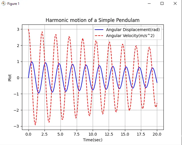
The above plot shows us that the angular velocity and the displacement is decresing gradually due to the effect of the damping which is provided as the input.

ANIMATION VIDEO:

Hence the animation and the plotting for the Second order ODE is completed successfully.

ERRORS:

Just some minor errors were made during the coding which are of the indentation which are solved accordingly else the errors were taken care of.