Week 3 - Solving second order ODEs

AIM: To write a program for simulating the transient behaviour of a simple pendulam.

OBJECTIVES:

• Simulate the transient behaviour of a simple pendulam
• Create an animation of its motion

GOVERNING EQUATION:

THEORY:

In Mathematics an ordinary differentian equation is a differential equation containing one or more functions of one independent variable and the derivatives of those functions.

ODE is used to derive the transient behaviour of a system. A simple pendulam is the basic example of the ODE. The way pendulam moves is in accordance to the Newtons law of motion and when it is written down in the mathematical formula we get the second order differential equation that describes the position of ball w.r.t time.

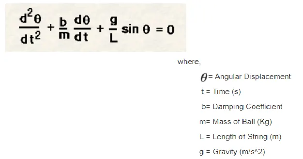
The above equation shows us the 2nd order differential equation of simple pendulam with damping.

THEORY:

In Mathematics an ordinary differentian equation is a differential equation containing one or more functions of one independent variable and the derivatives of those functions.

ODE is used to derive the transient behaviour of a system. A simple pendulam is the basic example of the ODE. The way pendulam moves is in accordance to the Newtons law of motion and when it is written down in the mathematical formula we get the second order differential equation that describes the position of ball w.r.t time.

The above equation shows us the 2nd order differential equation of simple pendulam with damping.

INPUT PARAMETERS FOR PROGRAMMING:

• Length of pendulam, l= 1m,
• Mass of ball, m=1kg,
• Damping coefficient, b=0.05
• Time span, = 0-20seconds
• Angular displacement = 0
• Angular velocity= 3rad/sec

STEPS WITH CODE:

Initially we have to define a function for ordinary differential equation for the pendulam so that in the main program we can call it and we can get to solve our equation for the simple pendulam and we can have its animation.

Function code:

function[dtheta_dt]=ode_func(t,theta,b,g,l,m)

theta1= theta(1)
theta2= theta(2)

% Defining the first ODE

dtheta1_dt=theta2;

% Defining the second ODE

dtheta2_dt = -(b/m)*theta2-(g/l)*sin(theta1);

dtheta_dt =[dtheta1_dt;dtheta2_dt];
end

In the above code we are defining the function which has 6 inputs in it starting with t(time), theta, b(damping coefficient), g(gravity), l(length of pendulam), m(mass) and then in the second line we are defining our values so that we can solve our main differential equation by dividing them into parts for ease calculation.

dtheta_dt is nothing, it is just dθ/dt so nothing to get confused here.

secondly after defining the second order ode, atlast we will combine them in a solution array of the name dtheta_dt with a (;) in it because the solution is going to be a column matrix.

Now we can proceed to our main programming code to solve the equation as follows:

Main Program Code:

clear all
close all
clc


% Input Variables
%Damping coefficient
b= 0.05;

% Gravity
g=9.81;

%Length of pendulam
l=1;

% Mass of ball
m=1;

%Initial conditions

theta_0 =[0;3];

% Time span

t_span= linspace(0,20,500);

% solving ode

[t,results]= ode45(@(t,theta)ode_func(t,theta,b,g,l,m),t_span,theta_0);

% Plotting
plot(t,results(:,1))
hold on
plot(t,results(:,2))
xlabel('time')
ylabel('Angular displacement')
title('Simple pendulam')

% Pendulam motion
x=0;
y=0;

for i=1:length(t)
    angle= results(:,1)
    ANGLE= angle(i);
    x1= sin(ANGLE)
    y1= -cos(ANGLE)
    figure(2)
    plot(x1,y1,'.','markersize',50)
    hold on
    plot([x x1],[y y1],'linewidth', 3)
    axis([-2 2 -1.5 1.5])
    hold off
    M(i)=getframe(gcf);
end

% creating simulation movie
movie(M)
videofile= VideoWriter('Pendulam_Motion')
open(videofile)
writeVideo(videofile,M)
grid on
close(videofile)

• In the main program the value of each input is assigned as of the b,g,l,m.
• the value of theta_0 which is assigned as [0;3] means here angular displacement is 0 and the angular velocity is 3 as required for the calculation
• The timespan means the time interval which is 0 to 20 seconds having 500 values in between them.
• After that we will write the code to solve our equation starting with an array of [t,results] means all the values will come out as an array and also we will use the ode45 and the function code which we made earlier.
• The ode45 is a function in MATLAB which solves ordinary or partial differential equations using a numerical method.
• To solve an ODE we need to integrate and solve for the variable which is done by calling the function and at last providing the initial conditions which needs to be integrated.
• After running this code we can get our results, to plot these results next plotting code is used which will plot both the result 1 and result 2 i.e of the displacement and the velocity of the pendulam by using the hold on command because without it the MATLAB will only execute the recent plot.
• When the plotting is done we need to create the animation of the pendulam for that the for loop is used so that for a particular value we can get our answers.
• While in the for loop we have to capture the frame by using the getframe command and at the end we will save our simulation movie of the title Pendulam_motion.

RESULTS:

The plot for the displacement and velocity which we get by solving our equation is as follows:

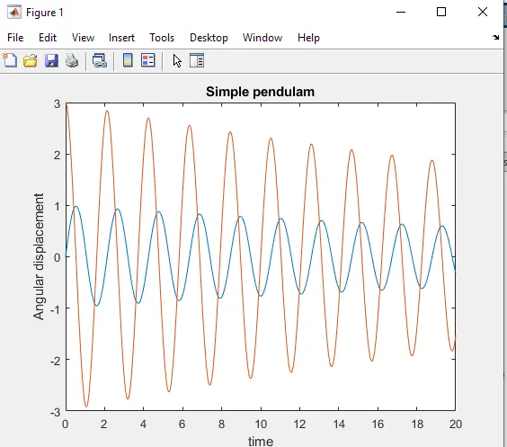
In the above graph we can see that the red lines shows us the angular velocity as it is starting from the value of 3 which we provided as the input and the blue line shows us the angular displacement as it is starting from the 0 which is our input value.

The animation video which we obtained is :

The pendulam is working perfectly as it can be seen in the video, it is according to our input variables.

ERRORS:

Just some minor mistakes were made while programming the code and it was corrected accordingly.

Hence this was the method to solve the second oder differential equation for simple pendulam.