Challenge

Week 3 - Solving second order ODEs

RRushikesh Khondekar17 Jun 2021

Aim:

To write the program for the ODE equation for a simple pendulum with damping and simulate it and create the animation.

Theory:

Ordinary differential equations:

In mathematics, an ordinary differential equation (ODE) is a differential equation containing one or more functions of one independent variable and the derivatives of those functions. The term ordinary is used in contrast with the term partial differential equation which may be with respect to more than one independent variable.

Simple Pendulum:

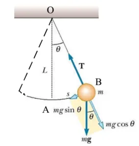
A pendulum is a weight suspended from a pivot so that it can swing freely. When a pendulum is displaced sideways from its resting, equilibrium position, it is subject to a restoring force due to gravity that will accelerate it back toward the equilibrium position. When released, the restoring force acting on the pendulum's mass causes it to oscillate about the equilibrium position, swinging back and forth.

The time for one complete cycle, a left swing, and a right swing is called the period. The period depends on the length of the pendulum and also to a slight degree on the amplitude, the width of the pendulum's swing.

Equation used:

The second-order ODE for a simple pendulum,

`(d^2t)/dt^2+b/m*(d(theta))/dt+g/L*sin(theta)=0` ----------(1)

where,

b: Damping Coefficient

m: mass of the ball

g: Gravitational force

L: Length of string

To change the ODE equation from 2nd order to 1st order,

let,

`theta=theta1`

put this in equation(1), we get,

`(d(theta))/dt=(d(theta1))/dt=theta2` ----------(2)

`(d^2(theta))/dt^2=(d^2(theta1))/dt^2=d/dt((d(theta1))/dt)=d/dt(theta2)` ----------(3)

put equation(2) & (3) in equation(1),

`(d^2(theta))/dt^2+b/m*(d(theta))/dt+g/L*sin(theta)=0`

`(d^2(theta1))/dt^2+b/m*(d(theta1))/dt+g/L*sin(theta1)`

`(d(theta2))/dt+b/m*(theta2)+g/L*sin(theta1)=0`

from this equation here we get two ODE equations,

`(d(theta1))/dt=theta2`

`(d(theta2))/dt=-b/m*theta2-g/Lsin(theta1)`

To arrange it in the matrix form,

`(d(theta))/dt=d/dt[[theta1],[theta2]]=[[theta2],[-b/m*theta2-g/Lsin(theta1)]]`

Terms used:

Ode45:

ode45 is a versatile ODE solver and is the first solver you should try for most problems. However, if the problem is stiff or requires high accuracy, then there are other ODE solvers that might be better suited to the problem

To solve an ODE, we have to integrate and solve for the variable. Assuming we have an ode du, we would solve for u by integrating du provided some limits of integration. However, rather than direct integration, we can use a numerical solver, by discretizing the equation, that is, we convert the ODE into a linear equation and then solve this equation to approximate the solution.

This function must then be input to ode45 as

[t,results] = ode45(@(t,y) ode(t,y,args), tspan, y0)

Procedure:

Starting from initial inputs such as clear all, close all, and clc and some inputs values of Damping coefficient, Gravitational force of the earth, Length of string, and Mass of the ball.

clear all 
close all 
clc

%Inputs values 
l = 1;     %Length of the string, mm
b = 0.05;  %Damping coefficient
m = 1;     %Mass of ball, kg
g = 9.81;  %Gravitational force of earth, m/sec^2

The angular displacement and angular velocity are given as initial conditions.

%Initial condition
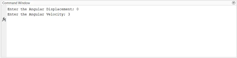
Angular_displacement = input('Enter the Angular Displacement; ');
Angular_Velocity = input('Enter the Angular Velocity; ');
theta_0 = [0,3];

Time is given from 0 to 20 secs and 500 frames in between it. That means time is equally divided from 0 to 20 secs up to 500 times.

%Time points
t_span = linspace(0,20,500);

The ODE function is created by using the ODE Equation,

function [dtheta_dt] = ode_func(t, theta,b,g,l,m)
    
    theta1= theta(1);
    theta2= theta(2);
    dtheta1_dt = theta2;
    dtheta2_dt = -(b/m)*theta2 - (g/l)*sin(theta1);
    dtheta_dt = [dtheta1_dt; dtheta2_dt];
end

The function is called along with time and theta.

%Solve ODE 

[t, results] = ode45(@(t,theta) ode_func(t, theta, b,g,l,m),t_span, theta_0);

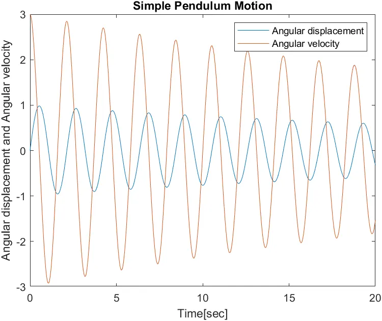
The graph is plotted for Angular Velocity and Angular Displacement vs Time.

%Plotting on graph
figure(1)
plot(t, results(:,1));
hold on;
plot(t,results(:,2));
title('Simple Pendulum Motion');
ylabel('Angular displacement and Angular velocity');
xlabel('Time[sec]');
legend('Angular displacement','Angular velocity')

To simulate the plot by using a for loop to continuously plot the graph of the pendulum.

%Simulation of pendulum
count = 1;

for i=1:length(results(:,1))
    x0= 0;
    y0= 0;
    x1= l*sin(results(i,1));
    y1= -l*cos(results(i,1));
    
    figure(2)
    plot([-0.5 0.5],[0, 0],'linewidth',3,'color','b');
    line([x0 x1],[y0 y1],'linewidth',2,'color','r');
    hold on;
    
    plot(x1,y1,'o','markers',20,'markerfacecolor','g');
    grid on;
    title('Simple Pendulum Motion');
    axis([-1.5 1.5 -1.5 0.5]);
    pause(0.01);
    hold off;
    M(count) = getframe(gcf);
    count =count +1;
end

Created the animation movie in AVI format by using the VideoWriter command.

%Creating movie
movie(M);
videofile = VideoWriter('pendulum_animation.avi', 'uncompressed AVI');
open(videofile);
writeVideo(videofile,M);
close(videofile);

Code:

Main code:

clear all 
close all 
clc

%Inputs values 
l = 1;     %Length of the string, mm
b = 0.05;  %Damping coefficient
m = 1;     %Mass of ball, kg
g = 9.81;  %Gravitational force of earth, m/sec^2

%Initial condition
Angular_displacement = input('Enter the Angular Displacement; ');
Angular_Velocity = input('Enter the Angular Velocity; ');
theta_0 = [0,3];

%Time points
t_span = linspace(0,20,500);

%Solve ODE 

[t, results] = ode45(@(t,theta) ode_func(t, theta, b,g,l,m),t_span, theta_0);

%Plotting on graph
figure(1)
plot(t, results(:,1));
hold on;
plot(t,results(:,2));
title('Simple Pendulum Motion');
ylabel('Angular displacement and Angular velocity');
xlabel('Time[sec]');
legend('Angular displacement','Angular velocity')

%Simulation of pendulum
count = 1;

for i=1:length(results(:,1))
    x0= 0;
    y0= 0;
    x1= l*sin(results(i,1));
    y1= -l*cos(results(i,1));
    
    figure(2)
    plot([-0.5 0.5],[0, 0],'linewidth',3,'color','b');
    line([x0 x1],[y0 y1],'linewidth',2,'color','r');
    hold on;
    
    plot(x1,y1,'o','markers',20,'markerfacecolor','g');
    grid on;
    title('Simple Pendulum Motion');
    axis([-1.5 1.5 -1.5 0.5]);
    pause(0.01);
    hold off;
    M(count) = getframe(gcf);
    count =count +1;
end
%Creating movie
movie(M);
videofile = VideoWriter('pendulum_animation.avi', 'uncompressed AVI');
open(videofile);
writeVideo(videofile,M);
close(videofile);

For function:

function [dtheta_dt] = ode_func(t, theta,b,g,l,m)
    
    theta1= theta(1);
    theta2= theta(2);
    dtheta1_dt = theta2;
    dtheta2_dt = -(b/m)*theta2 - (g/l)*sin(theta1);
    dtheta_dt = [dtheta1_dt; dtheta2_dt];
end

Result:

The plot is generated between Angular Displacement, Angular Velocity, and time.

The animation is generated for the simple pendulum in the required format.

The output is shown below: