Week 3 - Solving second order ODEs

Aim

To simulate a motion of a simple pendulum by solving second order differential equation in Matlab.

Theory

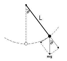
The figure shows an idealized pendulum with a massless string of length L and a bob of mass m. The open circle indicates the initial position of the bob. When the bob is moved from its rest position, it swings back and forth. The primary forces acting on the bob are the gravitational force that makes it move in the first place and the force exerted by the string to keep it moving along a circular path. In addition, there may be a damping force from friction at the pivot or air resistance or both. We will construct a model to describe how the angle of the pendulum varies as a function of time t. Let θ(t) be the corresponding angle with respect to the vertical. The figure shows tangential and radial components of gravitational force on the pendulum bob. Let s(t) be the distance along the arc from the lowest point to the position of the bob at time t, with displacement to the right considered positive.

s = L*θ

Adding damping to the model:

Program for solving second order differential equation

clear all
close all
clc

%input parameters
b = 0.05;
g = 9.81;
l = 1;
m = 1;

%initial condition
theta_0 = [0;3];

%time points
t_span = linspace(0,20,300);

[t,results] = ode45(@(t,theta) ode_func(t,theta,b,g,l,m),t_span,theta_0)
ct = 1;

%plotting
plot(t,results(:,1))
hold on
plot(t,results(:,2))
ylabel('plot')
xlabel('time')

% simulation of pendulum

for i = 1:length(results(:,1))
    x0 = 0;
    y0 = 0;
    x1 = l*sin(results(i,1));
    y1 = -l*cos(results(i,1));
    figure(2);
    plot([-1,1],[0,0],'linewidth',3,'color','r')
    line([x0 x1],[y0 y1],'linewidth',3,'color','g')
    hold on
    plot(x1,y1,'marker','o','markerSize',20,'markerFacecolor','g');
    axis([-2 2 -2 2]);
    grid on 
    pause(0.01)
    hold off
    M(ct) = getframe(gcf);
    ct = ct + 1;
end
movie(M);
videofile = VideoWriter('motion_of_pendulum.avi','uncompressed AVI')
open(videofile)
writeVideo(videofile,M)
close(videofile)

CODE EXPLANATION

• Define the given parameters and input
• The time span of 20 seconds is set using linspace command with 100 points between them.
• The theta values are given as a column matrix
• To solve the ode, ode45, a built-in function of Matlab which takes 3 inputs such as theta, t and the function ode_func.

ode_func script

function [dtheta_dt] = ode_func(t,theta,b,g,l,m)
theta1 = theta(1);
theta2 = theta(2);
dtheta1_dt = theta2;
dtheta2_dt = -(b/m)*theta2-(g/l)*sin(theta(1));

dtheta_dt = [dtheta1_dt;dtheta2_dt];
end

• Now use the plot command to plot graph.
• All images obtained are stored using getframe(gcf)
• The movie obtained is saved in a specific format using writeVideo command.

OUTPUT

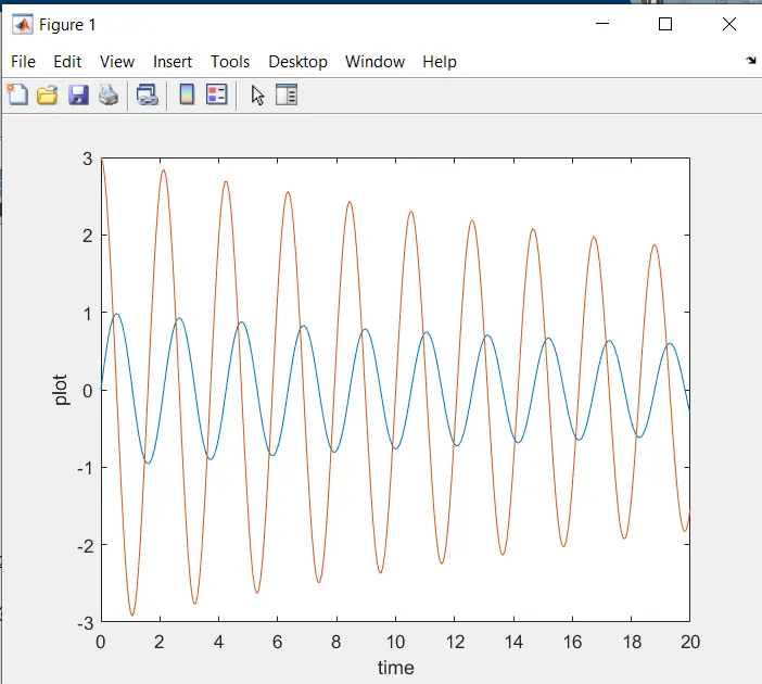
Video:

https://youtu.be/6XPO2biisxM

RESULTS

A Matlab program is written to animate the motion of a simple pendulum governed by second-order ode.