Solving second order ODEs

OBJECTIVE:

Write a program to solve the ODE and simulate the motion of a simple pendulum with damping.

PRE-REQUISITES:

i) In Engineering, ODE is used to describe the transient behavior of a system. A simple example is a pendulum.

ii) The way the pendulum moves depends on Newton's second law.

iii) When this law is written down, we get a second order Ordinary Differential Equation that describes the position of the "ball" w.r.t time.

iv) This ODE represents the equation of motion of a simple pendulum with damping:

`(d^2theta)/dt^2+b/m``(d theta)/dt+g/l*sintheta=0`

PROCEDURE:

a) Main Program:

i) Start with the inputs such as the damping coefficient, acceleration due to gravity, length of the pendulum, and mass of the ball.

ii) Now define the initial conditions of angular displacement and the angular velocity in a variable 'theta_0'.

iii) Now with the variable 't_span' the time span of the motion of the pendulum is defined using the 'linspace' command which divides the range of 0 to 20 in 500 equal intervals.

iv) Now the ODE is solved using the ODE solver that is inbuilt in Matlab i.e. “ode45”.

v) The syntax of 'ode45' is first we define the independent and the dependent variable '(t,theta)' then the function is called that contains the ODE.

vi) This function is integrated for getting the results 'ode_function(t,theta,b,g,l,m)' and then the time span is given for which the function is integrated 't_span' and then lastly the initial condition is given from which the calculation starts 'theta_0'.

vii) Any ODE to be integrated by 'ode45' must be provided as a set of first-order ODEs.

viii) All the results are stored in an array '[t, results]'.

ix) Create animation from the pendulum plots using the movie and VideoWriter command.

clear all
close all
clc

%Inputs
b = 0.05; 
g = 9.81;
l = 1;
m = 0.1;

%Initial condition
theta_0 = [0;5];

%Time points
t_span = linspace(0,10,500);

%Solving using ODE45
[t , results] = ode45(@(t,theta) ode_func(t, theta, b, g, l, m), t_span, theta_0);

%Plotting
plot(t,results)

%animation of pendulum movement
c=1;
for i=1:length(results(:,1))
    x0=0; %initial position
    y0=0; %initial position
    x1=l*sin(results(i,1)); 
    y1=-l*cos(results(i,1)); 
    
    %plotting the animation 
    subplot(5,3,[1:9])
    plot([-l l],[0 0],'linewidth',4,'color','k') 
    hold on
    line([x0 x1],[y0 y1],'linewidth',2,'color','b') 
    plot(x1,y1,'o','markersize',20,'markerfacecolor','r') 
    grid on
    axis ([-1.2 1.2 -1.2 0.2])
    pause (0.1)
    hold off
    M(c)=getframe(gcf);
    c=c+1;   
end
movie(M)
videofile=VideoWriter('Pendulum_Motion.avi','Uncompressed AVI');
open(videofile)
writeVideo(videofile,M)
close(videofile)

b) Function Program:

i) The name of the function and the name of the file should be the same or else the program will not run.

ii) Now the second-order ODE is broken into two first-order ODEs, first one to be 'dtheta1_dt' and the second to be 'dtheta2_dt'.

iii) Now the two results are combined in an array 'dtheta_dt' which contains values in two rows.

function [dtheta_dt] = ode_func(t, theta, b, g, l, m)
theta1 = theta(1);
theta2 = theta(2);
dtheta1_dt = theta2;
dtheta2_dt = -(b/m)*theta2 - (g/l)*sin(theta1)
dtheta_dt = [dtheta1_dt; dtheta2_dt]
end

RESULTS:

i) The following plot is obtained representing the damping:

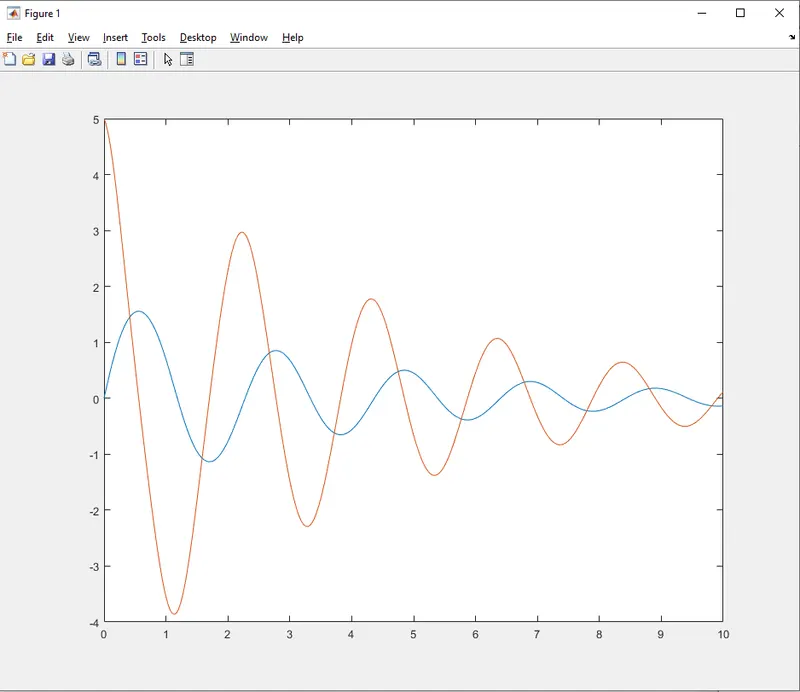
ii) The following video is created in '.avi' format representing the motion of a simple pendulum:

CONCLUSION:

i) Studied ODE functions and the methodology followed to solve them.

ii) Studied and implemented ode45 function.