Week 3 - Solving second order ODEs
- Pendulum move simulation and Upload an animation on Youtube and provide the Youtube link for animation in your report.
DETAILED REPORT:
AIM:
- Write Matlab code to plot pendulum move simulation and Upload an animation on Youtube and provide the Youtube link for animation in your report.
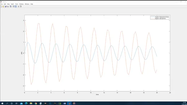
and damping graph
GOVERNING EQUATIONS :
OBJECTIVES OF THE PROJECT:
- Pendulum move simulation and Upload an animation on Youtube and provide the Youtube link for animation in your report.
- Damping graph
THEORY:
A simple pendulum consists of a point mass suspended from perfectly rigid support by a weightless , inextensible ,twistless and perfectly flexible fibre . a heavy metal sphere having very little radius then the length of fibre can be treated as a point mass. This metal sphere is called the bob of simple pendulum. The distance between the point of suspension up to the center of gravity of the bob is called the length of the simple pendulum.
Predefine parameter:
L=1 metre,
m=1 kg,
b=0.05.
g=9.81 m/s2.
Simulate the motion between 0-20 sec, for angular displacement=0,angular velocity=3 rad/sec at time t=0.
APPLICATION USED :
Matlab
CODE FOR CALCULATION AND EXPLANATION (ode_main.m) :
clear all
close all
clc
%damping coefficient
b=0.05;
%gravity
g=9.81;
%length
l=1;
%mass
m=1.0;
%initial condition
theta_0=[0 3];
%time points
t_span=linspace(0,20,100);
%solve ODE
[t,results]=ode45(@(t,theta)ode_func(t,theta,b,g,l,m),t_span,theta_0);
pos=results(:,1);
%now we plot the link
%here we use loop for every end value of link 1
ct=1;
for i=1:length(pos)
THETA1=pos(i);
%at origin
x0=0;
y0=0;
%at first link end
x1=l*sin(THETA1);
y1=-l*cos(THETA1);
%now we are plotting
plot([x0 x1],[y0 y1],x1,y1,'g.','markersize',30,'linewidth',5)
axis([-2.0 2.0 -2.0 2.0])
%title of plot
title('Solving second order ODEs by Rupal Deshmukh')
%add variable value at x label and y label as coordinates position
xlabel(['link 1 end coordinates X1= ' num2str(x1),' & Y1 =', num2str(y1)])
hold off
grid on
%pause video
pause(0.1)
%getting frames
M(ct) = getframe(gcf);
ct = ct+1;
end
%writing video
movie(M,1,5)
videofile=VideoWriter('odesecond');
%frame rate control in saved avi file
videofile.FrameRate = 5;
open(videofile)
writeVideo(videofile,M)
close(videofile)
figure(1)
plot(t,results(:,1))
hold on
plot(t,results(:,2))
ylabel('plot')
xlabel('time')
hold off;
axis ([0 22 -3.5 3.5])
legend('angular displacement/time','angular velocity/time')
Here function ode_func.m
function[dtheta_dt]=ode_func(t,theta,b,g,l,m)
theta1=theta(1)
theta2=theta(2)
dtheta1_dt=theta2;
dtheta2_dt=-(b/m)*theta2-(g/l)*sin(theta1);
dtheta_dt=[dtheta1_dt;dtheta2_dt];
end
5.CONCLUSION:
- Pendulum move simulation and Upload an animation on You tube and provide the You tube link for an animation in your report.
https://youtu.be/VNZRoiGXDWI
- Damping graph