Project 2 - Rankine cycle Simulator
DETAILED REPORT:
AIM:
- Create a Rankine Cycle Simulator using OCTAVE/MATLAB.
- Your code should calculate the state points of the Rankine Cycle (any type of your choice) based on user inputs.
- Then, plot the corresponding T-s and h-s plots for the given set of inputs. Title and axes labels are a must, while legends could be used if necessary.
- The presentation of your code will be taken into consideration while grading. Labelling sections of your code using comments is appreciated.
- Attach a report explaining the working of a rankine cycle simulator and also the research done by you.
THEORY:
What are Rankine Cycle?
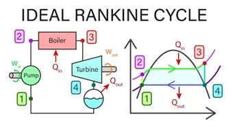
The Rankine cycle is an idealized thermodynamic cycle describing the process by which certain heat engines, such as steam turbines or reciprocating steam engines, allow mechanical work to be extracted from a fluid as it moves between a heat source and heat sink.
The ideal Rankine cycle consists of the following four processes, as shown on the T-s diagram on the left: 1-2: Isentropic compression in a pump. 2-3: Constant pressure heat addition in a boiler. ... 4-1: Constant pressure heat rejection in a condenser.
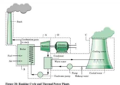
The Rankine cycle or Rankine Vapor Cycle is the process widely used by power plants such as coal-fired power plants or nuclear reactors. In this mechanism, a fuel is used to produce heat within a boiler, converting water into steam which then expands through a turbine producing useful work.
APPLICATION USED :
Matlab
CODE FOR CALCULATION AND EXPLANATION (rankine_cycle.m) :
firstly download or copy XSteam file in active directory of main file.
clear all
close all
clc
disp('RANKINE CYCLE');
disp('1-2 is isentropic expansion in the turbine');
disp('2-3 is constant pressure heat removal in the condenser');
disp('3-4 is isentropic compression in the pump');
disp('4-1 is constant pressure heat addition in the boiler');
%obtaining the input data
p1 = input('nValue of pressure at turbine inlet ,p1(in bar)=');
T1 = input('nValue of temperature at turbine inlet ,T1(in degree.C)=');
p2 = input('nValue of temperature at condenser inlet ,p2(in bar)=');
%Extracting data_defining variables
%state 1 ( extracting enthalpy at state pt 1 and similarly)
h1 = XSteam('h_pT', p1, T1);
s1 = XSteam('s_pT', p1, T1);
%at state 2
s2 = s1;
sf2 = XSteam('sL_p',p2);
sg2 = XSteam('sV_p',p2);
x2 = (s2-sf2)/(sg2-sf2);
hf2 = XSteam('hL_p',p2);
hg2 = XSteam('hV_p',p2);
h2 = hf2 +(x2*(hg2-hf2));
%at state 3
p3 = p2;
s3 = XSteam('sL_p',p3);
h3 = XSteam('hL_p',p3);
%at state 4
s4 = s3;
p4 = p1;
%work done yo
Wt = h1-h2;
%work done to run pump
v3 = XSteam('vL_p',p3);
Wp = v3*(p4 - p3)*100;
h4 = h3 + Wp;
%net Work
Wnet = Wt - Wp;
%Heat into the system
Qin = h1 - h4;
%Heat out of the system
Qout = h2 - h3;
%Thermal effieciency
eff = (Wnet/Qin)*100;
%specific steam Consumtion = mass flow rate/power
SSC = (3600/Wnet);
% calculating temperature ar the state points
T3 = XSteam('Tsat_p',p3);
T2 = T3;
Cp4 = XSteam('Cp_ps',p4,s4);
Cv4 = XSteam('Cv_ps',p4,s4);
k = Cp4/Cv4;
T4 = T3/((p3/p4)^((k-1)/k));
% calculating temperature entropy and enthalpy at the vapour and liquid
% line for ploting
T6 = XSteam('Tsat_p',p1);
s5 = XSteam('sL_p',p1);
s6 = XSteam('sV_p',p1);
h5 = XSteam('hL_p',p1);
h6 = XSteam('hV_p',p1);
T5 = T6;
%ploting the saturation curve
T = linspace(1,375,1000);
for i = 1:length(T)
sf(i) = XSteam('sL_T',T(i));
sg(i) = XSteam('sV_T',T(i));
hf(i) = XSteam('hL_T',T(i));
hg(i) = XSteam('hV_T',T(i));
end
%plotting T-S diagram
figure(1)
hold on
plot(sf,T,'r','linewidth',1)
plot(sg,T,'r','linewidth',1)
plot([s1 s2],[T1 T2],'k','linewidth',2)
plot([s2 s3],[T2 T3],'k','linewidth',2)
plot([s3 s4],[T3 T4],'k','linewidth',2)
plot([s4 s5],[T4 T5],'k','linewidth',2)
plot([s5 s6],[T5 T6],'k','linewidth',2)
sc1 = linspace(s6, s1,1000);
for l = 1:length(sc1)
Tc1(l) = XSteam('T_ps',p1,sc1(l));
end
plot(sc1, Tc1, 'k', 'linewidth', 2)
text(s1+0.1, T1, '1')
text(s2+0.1, T2, '2')
text(s3, T3-20, '3')
text(s4, T4+20, '4')
title('Temp vs entropy plot')
xlabel('entropy ,S(Kj/kgk)')
ylabel('temperature(degree C)')
legend('saturation curve')
% plotting h-s diagram
figure(2)
hold on
plot(sf, hf,'r','linewidth',1)
plot(sg, hg,'r','linewidth',1)
plot([s1 s2],[h1 h2],'k','linewidth',2)
plot([s2 s3],[h2 h3],'k','linewidth',2)
plot([s3 s4],[h3 h4],'k','linewidth',2)
hc = linspace(h4, h5,100);
for k = 1:length(hc)
sch(k) = XSteam('s_ph',p1,hc(k));
end
plot(sch, hc, 'k', 'linewidth', 2)
plot([s5 s6],[h5 h6],'k','linewidth',2)
for m = 1:length(sc1)
hc1(m) = XSteam('h_ps',p1,sc1(m));
end
plot(sc1, hc1, 'k', 'linewidth', 2)
text(s1+0.1, h1, '1')
text(s2+0.1, h2, '2')
text(s3, h3-100, '3')
text(s4, h4+200, '4')
title('Enthalpy vs entropy plot')
xlabel('entropy ,S(Kj/kgk)')
ylabel('Enthalpy ,H(Kj/kg)')
legend('saturation curve','location','northwest')
%backwork Ratio
BW=Wp/Wt;
%displaying Results
disp('RESULTS');
fprintf('At state Point 1 \n');
fprintf('p1: %8.3f barn',p1);
fprintf('\n');
fprintf('T1: %8.3f Cn',T1);
fprintf('\n');
fprintf('h1: %8.3f Kj/Kgn',h1);
fprintf('\n');
fprintf('s1: %8.3f Kj/KgKnn',s1);
fprintf('\n\n\n');
fprintf('At State Point 2 \n');
fprintf('p2: %8.3f barn',p2);
fprintf('\n');
fprintf('T2: %8.3f Cn',T2);
fprintf('\n');
fprintf('h2: %8.3f Kj/Kgn',h2);
fprintf('\n');
fprintf('s2: %8.3f Kj/KgKnn',s2);
fprintf('\n');
fprintf('x2: %8.3f fnn',x2);
fprintf('\n\n\n');
fprintf('At State Point 3 \n');
fprintf('p3: %8.3f barn',p3);
fprintf('\n');
fprintf('T3: %8.3f Cn',T3);
fprintf('\n');
fprintf('h3: %8.3f Kj/Kgn',h3);
fprintf('\n');
fprintf('s3: %8.3f Kj/KgKnn',s3);
fprintf('\n\n\n');
fprintf('At State Point 4 \n');
fprintf('p4: %8.3f barn',p4);
fprintf('\n');
fprintf('T4: %8.3f Cn',T4);
fprintf('\n');
fprintf('h4: %8.3f Kj/Kgn',h4);
fprintf('\n');
fprintf('s4: %8.3f Kj/KgKnn',s4);
fprintf('\n\n\n');
fprintf('Turbine Work/ Net Work: %8.3f Kj/kgn',Wt);
fprintf('\n');
fprintf('Pump Work: %8.3f Kj/kgn',Wp);
fprintf('\n');
fprintf('Wnet: %8.3f Kj/kgn',Wnet);
fprintf('\n');
fprintf('Thermal Efficiency: %8.3f Percent n',eff);
fprintf('\n');
fprintf('S.S.C: %8.3f kJ/kWh',SSC);
fprintf('\n');
fprintf('Back Work Ratio: %8.3f',BW);
5.OUTPUT :
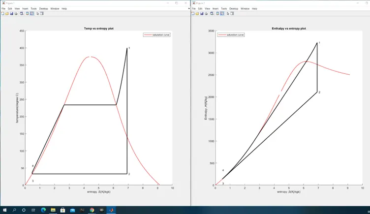
RANKINE CYCLE
1-2 is isentropic expansion in the turbine
2-3 is constant pressure heat removal in the condenser
3-4 is isentropic compression in the pump
4-1 is constant pressure heat addition in the boiler
nValue of pressure at turbine inlet ,p1(in bar) =30
nValue of temperature at turbine inlet ,T1(in degree.C) =400
nValue of temperature at condenser inlet ,p2(in bar) =0.050
RESULTS At state Point 1
p1: 30.000 barn
T1: 400.000 Cn
h1: 3231.571 Kj/Kgn
s1: 6.923 Kj/KgKnn
At State Point 2
p2: 0.050 barn
T2: 32.875 Cn
h2: 2110.708 Kj/Kgn
s2: 6.923 Kj/KgKnn
x2: 0.814 fnn
At State Point 3
p3: 0.050 barn
T3: 32.875 Cn
h3: 137.765 Kj/Kgn
s3: 0.476 Kj/KgKnn
At State Point 4
p4: 30.000 barn
T4: 36.935 Cn
h4: 140.776 Kj/Kgn
s4: 0.476 Kj/KgKnn
Turbine Work/ Net Work: 1120.863 Kj/kgn
Pump Work: 3.011 Kj/kgn
Wnet: 1117.852 Kj/kgn
Thermal Efficiency: 36.167 Percent n
S.S.C: 3.220 kJ/kWh
Back Work Ratio: 0.003