Week 3 - Solving second order ODEs

AIM:
Write a program in Python that will simulate the pendulum motion.

OBJECTIVES OF THE PROJECT:

for given differential equation which governs the motion of a simple pendulum undergoing simple harmonic motion (SHM) and make a pendulum animation using python.

THEORY:
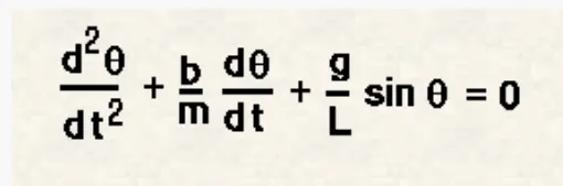
A simple pendulum consists of a point mass suspended from a perfectly rigid support by a weightless, inextensible, twistless, and perfectly flexible fiber. a heavy metal sphere
having a very less radius than the length of fiber can be treated as a point mass. This metal
sphere is called a bob of a simple pendulum. The distance between the point of suspension to
the center of gravity of the bob is called the length of the simple pendulum.

GOVERNING EQUATIONS :

Predefine parameter:

CODE with EXPLANATION :

import numpy as np;
from scipy.integrate import odeint;
import math;
import matplotlib.pyplot as plt;

#  importing library for video creation
import os
import cv2

# Importing library for merge png to gif
from PIL import Image;
import glob;


# Function that return dtheta/dt
def function(theta,t,b,g,l,m):
    theta1 = theta[0]
    theta2 = theta[1]
    dtheta1_dt = theta2;
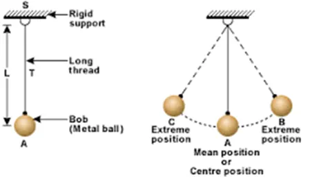
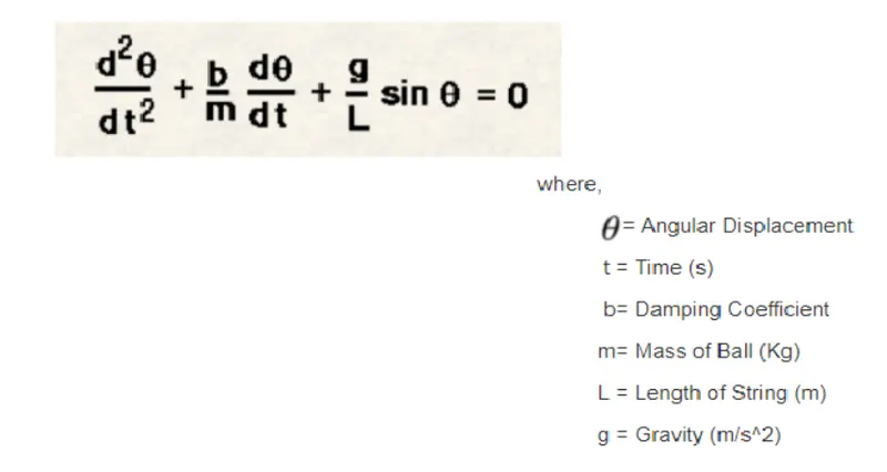
    dtheta2_dt = -(b/m)*theta2-(g/l)*math.sin(theta1);
    result = [dtheta1_dt,dtheta2_dt];
    return result

# Damping coffiecient
b = 0.05
# Acceleration due to gravity
g = 9.81;
# length of string
l = 1;
# mass of blob
m = 1;
# thetha_0 = [initial displacement , initial velocity]
theta_0 = [0,3]
# timespan 0-10 second
t= np.linspace(0,10,150)

# use odeint for calculation
theta = odeint(function,theta_0,t,args=(b,g,l,m))

# ploting the results
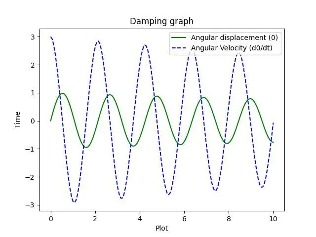
plt.plot(t,theta[:,0],'g-')
plt.plot(t,theta[:,1],'b--')

# add a legend  
plt.legend(['Angular displacement (0)',"Angular Velocity (d0/dt)"], loc ="upper right")

# labeling the axis
plt.xlabel("Plot")
plt.ylabel("Time")

# initialize title 
plt.title("Damping graph");

# initialize and save figure in current directory
fig = plt.gcf()
fig.savefig('Damping_graph.jpg')

plt.show();


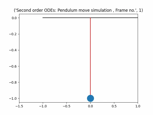
# Create pendulum animation
ct = 1
x0 = 0
y0 = 0

for i in theta[:,0]:
    x1=x0+(l*math.sin(i))
    y1=y0+(-l*math.cos(i))

    # initialize file name
    filename = str(ct)+'.png'
    ct = ct+1;

    # ploting pendulum
    plt.figure();
    # initialize black base line
    plt.plot([-1,1],[0,0],"black")
    # initialize pendulum string line
    plt.plot([x0,x1],[y0,y1],"red")
    # initialize pendulum blob
    plt.plot(x1,y1,'o',markersize = '20')

    # initialize title
    title = 'Second order ODEs: Pendulum move simulation , Frame no.', ct-1;
    plt.title(title);

    plt.xlim([-1.5,1.5])
    plt.xlim([-1.5,1.0])
    plt.savefig(filename)

# # ____________  save png files as video file _______

# get current folder location
image_folder = os.getcwd();

# initialize video name
video_name = 'video.avi'

# checking and selecting images in filder
images = [img for img in os.listdir(image_folder) if img.endswith(".png")]

# join one or more path components an write with cv moduule
frame = cv2.imread(os.path.join(image_folder, images[0]))
height, width, layers = frame.shape
video = cv2.VideoWriter(video_name, 0, 1, (width,height))

#  Sorting Image by name
sortedImages = sorted (images, key = lambda x: (len (x), x))

# initialize blank array for gif
gif_frames = []

# adding images into video
for image in sortedImages:
    video.write(cv2.imread(os.path.join(image_folder, image)))

    # for every images in directory for gif generation
    new_frame = Image.open(image)
    gif_frames.append(new_frame)

# Save fames into a GIF file 
gif_frames[0].save('Animation.gif', format='GIF',
               append_images=gif_frames[1:],
               save_all=True,
               duration=600, loop=1)

#  destroy or close all background functions
cv2.destroyAllWindows()

# save video 
video.release()

CONCLUSION:
• Pendulum move simulation

• Damping graph