Week 2 Air standard Cycle

AIM:

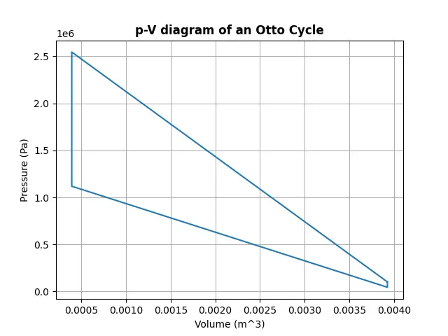
Write Python code to plot a PV diagram for otto cycle and calculate its thermal efficiency.

OBJECTIVES OF THE PROJECT:

• Plot a PV diagram for the otto cycle.
• Calculation of thermal efficiency.

THEORY:

The Otto cycle is the ideal cycle for spark-ignition (SI) engines. This cycle was presented in the late 19th century after Nikolaus Otto demonstrated the four-stroke SI engine successfully [1]. A description of the processes is given as follows:

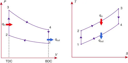
Process 1-2: isentropic compression of the working fluid occurs as the piston moves from bottom dead center (BDC) to top dead center (TDC).

Process 2-3: here, with the SI, a rapid burning occurs inside the piston; therefore, the heat addition takes place at the constant volume.

Process 3-4: in this process, the working fluid expands isentropically and produces useful work for the cycle.

Process 4-1: heat removal at constant volume. In practical applications, the heat is removed by expelling the exhaust gas to the atmosphere.

The Diesel cycle is used in numerous large-scale industrial applications for power generation. The Diesel engine is also known as a compression ignition (CI) engine, which was proposed in Germany by Rudolf Diesel in the late 19th century. In the CI engine, the ignition of the combustion process is attained by compression of the working fluid up to a larger temperature than the fuel’s autoignition temperature. When the temperature of the air increases adequately, high-pressure liquid fuel is sprayed into the combustion chamber. Thus, the ignition process occurs rapidly [1]. P-v and T-s diagrams of the ideal Diesel cycle are presented in Fig.

GOVERNING EQUATIONS :

• Ideal gas equation: PV=nRT

Here P = pressure (pascals)

V = volume (m^3)

n=mass of gas in (kg)

R=ideal gas constat (kJ/kg K)

T=temperature in kelvin (K)

• Volume at a particular instance in the engine cylinder (V)

V/V_c = 1 + ½ (r_c-1)[R+1-cosθ-(R²-(sinθ)²)^1/2]

Here V = Volume at a particular instance in the engine cylinder

V_c = Clearance Volume

r_c = Compression ratio

R = Length of connecting rod/crank pin radius

Θ = Crank Angle

• Isotropic process PV^γ = Constant
• The compression ratio of the otto cycle : r_c = V₁/V₂
• Thermal efficiency of otto cycle : η = 1-1/( r_c^γ-1)
• Volume swept V_s = π/4 x (diameter)² x stroke length
• Clearance volume V_{c =} V_s/ ( r_c -1)

Inputs

# Inputs are
gamma = 1.4
t3 = 2000
#  state 1 variable (at state 1 pressure is 1 atmosphere and temp 500k)
p1 = 101325
t1 = 350
#  engine Geometric parameters
bore = 0.15;
stroke = 0.2;
con_rod= 0.8;
cr = 10;

Code for calculation and explanation :

# case 1 : Plot between Velocity and Drag Force
import numpy as np;
import matplotlib.pyplot as plt;
import math;

# defining function for trace the volume for expansion and compression for varing crank angles
def engine_kinematics(bore,stroke,con_rod,cr,start_crank,end_crank):
    # engine geometric property
    a = stroke/2;
    R = con_rod/a;

    # volume parameter
    v_s = (math.pi/4)*pow(bore,2)*stroke;
    v_c = v_s/(cr-1);

    # start and end crank angle
    sc = math.radians(start_crank);
    ec = math.radians(end_crank);

    theta = np.linspace(sc,ec,50);
    v = [];
    for i in range (0,50):
        Theta = theta[i];
        term1 = 0.5*(cr-1);
        term2 = R + 1 - math.cos(Theta);
        term3 = pow(R,2)-pow(math.sin(Theta),2);
        term3 = pow(term3,0.5);
        v.append((1+ term1*(term2 - term3))*v_c);
    return v;

# Inputs are
gamma = 1.4
t3 = 2000
#  state 1 variable (at state 1 pressure is 1 atmosphere and temp 500k)
p1 = 101325
t1 = 350
#  engine Geometric parameters
bore = 0.15;
stroke = 0.2;
con_rod= 0.8;
cr = 10;

# calculating the swept volume and clearance volume
v_swept = (math.pi/4)*pow(bore,2)*stroke;
v_clearance=v_swept/(cr-1);
v1 = v_swept + v_clearance
v2 = v_clearance

# state variable at state point 2
# p2v2^gamma = p1v1^gamma
# p2=p1*(v1/v2)^gamma=p1*cr^gamma
p2=p1*pow(cr,gamma);

# p1v1/t1=p2v2/t2 
# t2 =p2*v2*t1/(p1*v1)
t2 = p2*v2*t1/(p1*v1);

# to find variation of volume during compression stroke as a function of crank angle theta;
V_comp = engine_kinematics(bore,stroke,con_rod,cr,180,0);
C_const = p1*pow(v1,gamma);
P_comp = [];

for v in V_comp:
    P_comp.append(C_const/pow(v,gamma))

# state variable at point 3
# pv/t = constant and for process 2-3 v2 = v3
# p2/t2 = p3/t3
p3 = p2*(t2/t3)
v3 = v2

# to find variation of volume during expansion  stroke as a function of crank angle theta
V_expp = engine_kinematics(bore,stroke,con_rod,cr,0,180);
C_const = p3*pow(v3,gamma);
P_expp = [];

for v in V_expp:
    P_expp.append(C_const/pow(v,gamma))

# Calculating p4 and v4 (isentropic expansion process)
# p3*v3^gamma = p4*v4^gamma
v4 = v1
p4 = p3*pow(v3,gamma)/pow(v4,gamma);

# Plotting Therotical diagram
plt.plot([v1,v2,v3,v4,v1],[p1,p2,p3,p4,p1]);
plt.xlabel('Volume (m^3)');
plt.ylabel('Pressure (Pa)');
plt.title('p-V diagram of an Otto Cycle',fontweight="bold");
plt.grid();
plt.show();

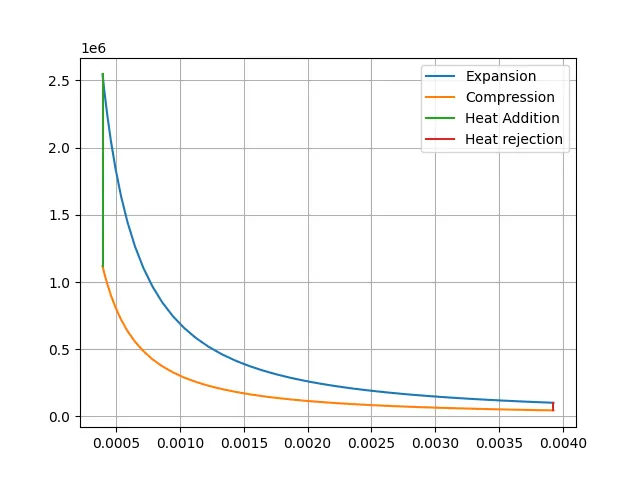
# plotting Actual diagram
plt.plot(V_comp,P_comp);
plt.plot(V_expp,P_expp);
plt.plot([v2,v3],[p2,p3]);
plt.plot([v4,v1],[p4,p1]);
# Function add a legend  
plt.legend(["Expansion","Compression", "Heat Addition","Heat rejection"], loc ="upper right")
plt.grid();
plt.show();

Result and Conclusion: