Week 3 - Solving second order ODEs

AIM:

To solve a second order differential equation using matlab.

GOVERNING EQUATIONS:

For a simple pendulum, a second order differential equation is used to describe the motion of the bob

`(d^2 θ)/(dt^2 )+b/m ( dθ)/dt+g/L sin⁡θ=0`

Where,

Θ = angular displacement of pendulum

t = time

b = damping coefficient

m= mass of the bob

g = acceleration due to gravity

To solve the second order differential equation it is converted to two first order differential equations as follows

Say

`θ= θ_1`

Then

`(dθ_1)/dt= θ_2`

`(dθ_2)/dt= -k/m θ_2-g/L sin⁡〖θ_1 〗`

Θ1 = angular displacement

Θ2 = angular velocity

OBJECTIVE:

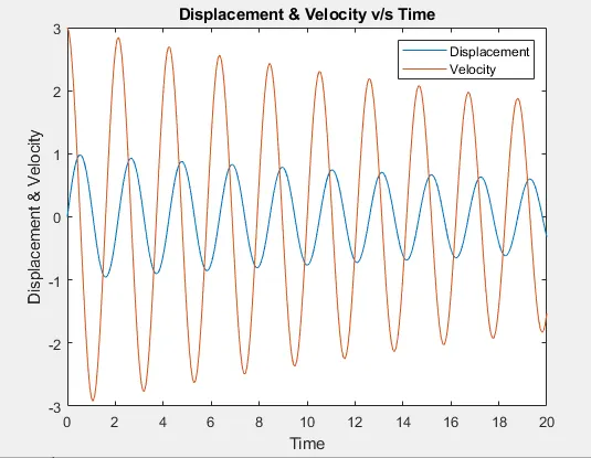
• To solve the ODE and plot displacement and velocity v/s time
• To simulate the motion of simple pendulum.

PROCEDURE:

1. Assign the given values of the physical parameters to the program.

b = 0.05

g = 9.81 m/s^2

m= 1 kg

l = 1 m

2. Prepare a sub function which shows the conversion of second order ODE into two first order ODE.
3. The initial condition of Θ1=0 and Θ2=3 and also the time span of 20 s is set into the program.
4. The ODE solver ode45 which is already defined in MATLAB is used to solve the program by calling the sub function to obtain the displacement and velocity
5. Plot the displacement and velocity v/s time.
6. Create a simulation of the motion of the pendulum

FUNCTION CODE:

function [dtheta_dt] = ode_func(t,theta,k,m,g,l)

theta1 = theta(1);
theta2 = theta(2);
dtheta1_dt = theta2;
dtheta2_dt = -(k/m)*theta2-(g/l)*sin(theta1);
dtheta_dt = [dtheta1_dt; dtheta2_dt];
end

Code Explanation:

The mathematical solution for converting the second order ODE to two first order ODE is shown in program.

MAIN CODE:

clear all
close all
clc

% input parameters
b= 0.05;
m = 1;
g = 9.81;
l = 1;

% initial conditions
theta_0 = [0;3];

% time points
t_span = linspace(0,20,300);

%solve ODE
[t results] = ode45(@(t,theta) ode_func(t,theta,b,m,g,l),t_span,theta_0);
 
% plotting graph
figure(1)
plot (t,results)
xlabel('Time')
ylabel('Displacement & Velocity')
legend('Displacement','Velocity')
title('Displacement & Velocity v/s Time') 

% stimulating animation
ct = 1;
for i = 1:length(results(:,1))
   
   x0 = 0;
   y0 = 0;
   
   x1 = l*sin(results(i,1));
   y1 = -l*cos(results(i,1));
   
   figure(2)
   plot([x0 x1],[y0 y1],'linewidth',3)
   hold on
   plot(x1,y1,'o','markersize',15,'markerfacecolor','r','markeredgecolor','b')
   hold off
   axis([-1 1 -1.5 0])
   pause(0.01)
   
   M(ct) = getframe(gcf);
   ct =ct+1;
   
end

% create video 
movie(M)
videofile = VideoWriter('ode_solution.avi','Uncompressed AVI');
open(videofile)
writeVideo(videofile,M)
close(videofile)

Code Explanation:

• Add physical parameters of the pendulum like length, mass, acceleration due to gravity and damping coefficient.
• Give the initial conditions and timespan for which you want to run the simulation
• Then use the ode solver ode45 function which main inputs as (t, theta) by calling the function ode_func with inputs (t,theta,l,b,g,m) and the initial conditions ast_span and theta_0
• The obtained results are stored in an array of [t,results]
• Since the results contain 2 components, angular displacement and velocity, to plot both the graphs, use the (:,1) and (:,2) and plot the graph.
• To create animation for loop so that we can get the x and y coordinates
• Use the pause() function to give a pause for every looping of values.
• Use movie making command as per code to create an animation.

PLOT:

ANIMATION:

https://drive.google.com/file/d/1s6qXoWMjG5szB79a-IskgECyqCPvi-fA/view?usp=sharing

CONCLUSION:

• The reduction in angle displacement and velocity is due to damping is due to the damping coefficient indroduced in the second order ODE of a simple pendulum.
• We have successfully solved the second order ODE