Project 2 - Rankine cycle Simulator

AIM:

1) To write a program that calculates the state points of a Rankine Cycle based upon user input of pressures at condenser and turbine and temperature at turbine.

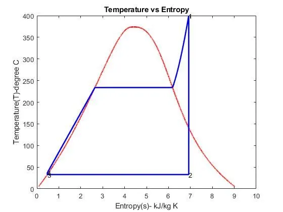
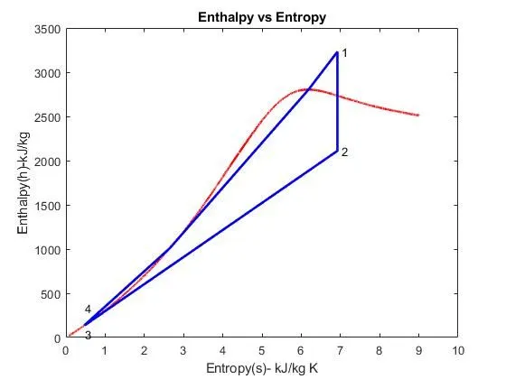
2) Plot T-S and H-S diagram for the corresponding values obtained.

THEORY:

Rankine cycle is a thermodynamic cycle that is used to convert heat produced by burning a fuel into mechanical energy. The Rankine cycle makes use of increase in pressure of a condensed fluid which is forced to vapourise in a vessel. The cycle begins when a fluid such as water is compressed under high pressure. This high pressure liquid is converted to vapour and this vapour is used to rotate a turbine which produces mechanical work. When the vapour is cooled, it turns into a liquid state and this cycle repeats.

The Rankine cycle makes use of 4 main components.

1. a) Pump: Used to compress liquid to high pressure and feed to the boiler.
2. b) Boiler: The boiler converts liquid/water to vapour state.
3. c) Turbine: The high pressure vapour in used to rotate turbine and convert heat to mechanical or electrical energy (by connecting the turbine to a generator).
4. d) Condenser: The condenser is used to cool the vapour and convert it to liquid state.

Rankine cycle include four processes

1. Process (1-2) :- Isentropic Expansion
2. Process (2-3) :- Isobaric Heat Rejection
3. Process (3-4) :- Isentropic Compression
4. Process (4-1) Isobaric Heat Transfer

REQUIRED FORMULAE:

1. `Q_a= h_1-h_4`
   Qa is heat addition
   h1 is enthalpy at state 1
   h4 is enthalpy at state 4
2. `W_t= h_1-h_2`
   Wt is work done by turbine
   h2 is enthalpy at state 2
3. `W_p= h_4-h_3`
   Wp is work done ny the pump
   h3 is enthalpy at state 3
4. Net Work Output
   `W_n = W_t-W_p`
5. Thermal Efficiency
   `η_t= (W_t-W_(p))/Q_a`
6. Back Work Ratio
   `BWR=W_p/W_t`
7. Specific Steam Consumption
   `SSC=3600/W_n`

CODE:

clear all
close all
clc

disp('process 1-2: Isentropic expansion ')
disp('process 2-3: constant pressure heat rejection')
disp('process 3-4: Isentropic Compression')
disp('process 4-1: constant pressure heat addition')

% Intial parameters
p1 = input('inlet pressure at turbine is ');
p2 = input('inlet pressure at condesor is ');
T1 = input('inlet temperature at turbine is ');

% State 1 parameters
Tsat = XSteam('Tsat_p',p1);
h1 = XSteam('h_pT',p1,T1);
s1 = XSteam('s_pT',p1,T1);

% State 2 parameters
s2 = s1;
sf2 = XSteam('sL_p',p2);
sg2 = XSteam('sV_p',p2);
hf2 = XSteam('hL_p',p2);
hg2 = XSteam('hV_p',p2);
x2 = (s2-sf2)/(sg2-sf2);
h2 = hf2 + x2*(hg2-hf2);
T2 = XSteam('T_ps',p2,s2);

% State 3 parameters
p3 = p2;
T3 = T2;
s3 = sf2;
h3 = hf2;

% State 4 parameters
s4 = s3;
p4 = p1;
h4 = XSteam('h_ps',p4,s4);
cp = XSteam('cp_ps',p4,s4);
cv = XSteam('cv_ps',p4,s4);
r = cp/cv;
T4 = T3*(p4/p3)^((r-1)/r);

% State 5 parameters
T5 = Tsat;
h5 = XSteam('hL_p',p1);
s5 = XSteam('sL_p',p1);

% State 6 parameters
T6 = T1;
h6 = XSteam('hV_p',p1);
s6 = XSteam('sV_p',p1);

% Plotting T-s Diagram
t1=linspace(5,400,25000);
for i=1:length(t1)
sf(i)=XSteam('sL_t',t1(i));
sg(i)=XSteam('sV_t',t1(i));
hf(i)=XSteam('hL_t',t1(i));
hg(i)=XSteam('hV_t',t1(i));
end

figure(1)
plot(sf,t1,'color','r','linewidth',2);
hold on
plot(sg,t1,'color','r','linewidth',2);

plot([s1,s2,s3,s4,s5,s6],[T1,T2,T3,T4,T5,Tsat],'color','b','linewidth',2);
text(s1, T1, '1')
text(s2, T2, '2')
text(s3, T3, '3')
text(s4, T4, '4')
title('Temperature vs Entropy')
xlabel('Entropy(S)- kJ/kg K')
ylabel('Temperature(T)-degree C')

% Plotting Superheated state
Ts=linspace(Tsat,T1,500);
for i=1:length(Ts)
    Ss(i)=XSteam('s_pt',p1,Ts(i));
end
plot(Ss,Ts,'linewidth',2,'color','b')
title('Temperature vs Entropy')
xlabel('Entropy(s)- kJ/kg K')
ylabel('Temperature(T)-degree C')

% Plotting h-s Diagram
figure(2)
plot(sf,hf,'color','r','linewidth',2);
hold on
plot(sg,hg,'color','r','linewidth',2);

plot([s1,s2,s3,s4,s5,s6,s1],[h1,h2,h3,h4,h5,h6,h1],'linewidth',2,'color','b');
text(s1+0.1, h1, '1')
text(s2+0.1, h2, '2')
text(s3, h3-100, '3')
text(s4, h4 +200, '4')
title('Enthalpy vs Entropy')
xlabel('Entropy(s)- kJ/kg K')
ylabel('Enthalpy(h)-kJ/kg')

% Result to be displayed in the command window 
disp(' The following are the results of rankine cycle operation ')
disp(' ')
disp(' At the state point 1')
disp(' ')
b1=sprintf('p1 is %.2f bar',p1);
disp(b1)
b2=sprintf('T1 is %.2f Deg Celcius',T1);
disp(b2)
b3=sprintf('h1 is %.2f kJ/kg',h1);
disp(b3)
b4=sprintf('s1 is %.2f kJ/kgK',s1);
disp(b4) 

disp(' ')
disp(' At the state point 2')
disp(' ')
b5=sprintf('p2 is %.2f bar',p2);
disp(b5)
b6=sprintf('T2 is %.2f Deg Celcius',T2);
disp(b6)
b7=sprintf('h2 is %.2f kJ/kg',h2);
disp(b7)
b8=sprintf('s2 is %.2f kJ/kgK',s2);
disp(b8) 

disp(' ')
disp(' At the state point 3')
disp(' ')
b9=sprintf('p3 is %.2f bar',p3);
disp(b9)
b10=sprintf('T3 is %.2f Deg Celcius',T3);
disp(b10)
b11=sprintf('h3 is %.2f kJ/kg',h3);
disp(b11)
b12=sprintf('s3 is %.2f kJ/kgK',s3);
disp(b12) 

disp(' ')
disp(' At the state point 4')
disp(' ')
b13=sprintf('p4 is %.2f bar',p4);
disp(b13)
b14=sprintf('T4 is %.2f Deg Celcius',T4);
disp(b14)
b15=sprintf('h4 is %.2f kJ/kg',h4);
disp(b15)
b16=sprintf('s4 is %.2f kJ/kgK',s4);
disp(b16)

% Workdone by turbine

W_D_T = h1-h2

% Workdone by the pump

W_D_Pump = h4-h3

%net workdone

W_D_Net = W_D_T-W_D_Pump

% Heat Supplied
qa = h1-h4;

% Effeciency
n = W_D_Net/qa

% Specific steam consumption
ssc = 3600/W_D_Net

% Back Work Ratio
BWR = W_D_Pump/W_D_T

Code Explanation:

1. Use clear all ; close all; clc; for clearing the windows with previous data and closing any previous figures/plots generated.
2. First, the four processes from 1-4 for Rankine cycle are printed using disp command.
3. The input parameters are defined using input command for T1, P1 & P2 variables.
4. Then extracting all the required values from the XSteam.m file library which act as a Standard Steam table to calculate the values for state points.
5. By using XSteam library file we call it by XSteam in MATLAB and the required function are taken and then giving the input accordingly to that particular function like in case of State point 1 input given is P1 & T1.
6. Similarly, state point 2, 3, & 4 are calculated for Enthalpy, Entropy, Pressure & Temperature using XSteam functions. Also the 5 and 6 state values are determined
7. Next using the basic formulae for Work done (W.D), Heat transferred (Qa) and thermal efficiency for the Rankine cycle is calculated.
8. Then, temperature range has been specified using linspace command & the corresponding of enthalpy and entropy are determined using for loop to plot saturation curve in figure 1.
9. After that Temperature v/s Entropy has been plotted in figure 1 using plot command by mentioning s1 to s4 for X-axis & T1 to T4 points for Y-axis along with the saturated curve.
10. A command named text is used further in last step for plotting the T-s graph in which text command is used add text descriptions to data points like 1,2,3 & 4 we had added easily.
11. Same procedure that is used to plot T-s graph is repeated and coded further for Enthalpy v/s Entropy graph to get the output.
12. In the final step all the calculated state points and the necessary values like net work done, efficiency, back ratio, etc had been printed step by step using fprintf command in command window.

RESULT:

• The following results are obtained in the command window

process 1-2: Isentropic expansion
process 2-3: constant pressure heat rejection
process 3-4: Isentropic Compression
process 4-1: constant pressure heat addition
inlet pressure at turbine is 30
inlet pressure at condesor is 0.05
inlet temperature at turbine is 400
The following are the results of rankine cycle operation

At the state point 1

p1 is 30.00 bar
T1 is 400.00 Deg Celcius
h1 is 3231.57 kJ/kg
s1 is 6.92 kJ/kgK

At the state point 2

p2 is 0.05 bar
T2 is 32.88 Deg Celcius
h2 is 2110.71 kJ/kg
s2 is 6.92 kJ/kgK

At the state point 3

p3 is 0.05 bar
T3 is 32.88 Deg Celcius
h3 is 137.77 kJ/kg
s3 is 0.48 kJ/kgK

At the state point 4

p4 is 30.00 bar
T4 is 36.94 Deg Celcius
h4 is 140.76 kJ/kg
s4 is 0.48 kJ/kgK

W_D_T = 1.120862815255960e+03
W_D_Pump = 2.997106658483858
W_D_Net = 1.117865708597476e+03
n = 0.361674170208850
ssc =3.220422607395944
BWR = 0.002673928171843

• The plots are also obtained
  
  
  
  

CONCLUSION:

• Rankine cycle is used in Thermal power plant so it is vital to understand as its help to calculate all the properties of the steam so that it gives ease to improve power output and efficiency of the plant.
• As water is the working fluid it is necessity to understand all its properties for this cycle, which we get to learn in this project.
• Setting/coding one program to calculate all the plots/figures and steam property at every stage of Rankin cycle will we easy for any one, as one have to put just three input, p1, T1 and p2, even non-technical person can simulate it.
• At last, this simulator help to reduce enormous amount of time to generate results.

REFERENCE:

https://en.wikipedia.org/wiki/Rankine_cycle#:~:text=The%20Rankine%20cycle%20is%20an,heat%20source%20and%20heat%20sink.

https://energyeducation.ca/encyclopedia/Rankine_cycle