Solving second order ODEs using MATLAB

THEORY

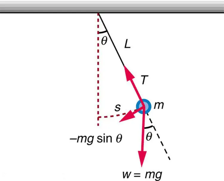
In Engineering, ODE is used to describe the transient behavior of a system. A simple example is a pendulum

The way the pendulum moves depends on the Newtons second law. When this law is written down, we get a second order Ordinary Differential Equation that describes the position of the "ball" w.r.t time.

Similarly, there are hundreds of ODEs that describe key phenomena and if you have the ability to solve these equations then you will be able to simulate any of theses systems.

Second Order Differential Equations are two

Homogeneous Second Order Differential Equations

• The first major type of second order differential equations you’ll have to learn to solve are ones that can be written for our dependent variable y and independent variable t as:
  
  `a*(d^2y)/dt^2+b*(dy)/(dt)+cy=0`
  
  
• Here a, b and c are just constants.

Inhomogeneous Second Order Differential Equations

• One extension to the above that we must tackle is the case when the RHS in our DE is non-zero, i.e. when we have:

`a*(d^2y)/dt^2+b*(dy)/(dt)+cy=f(t)`

OBJECTIVE

• To write a program that solves the following ODE. This ODE represents the equation of motion of a simple pendulum with damping

`(D^2theta)/(dt^2)+b/m*(d theta)/(dt)+g/l*sin(theta)=0`

CALCULATIONS

`(D^2theta)/(dt^2)+b/m*(d theta)/(dt)+g/l*sin(theta)=0` --> eq-1 we will be splitting this equation into 2

Assume -> `theta = theta1`

Then `(d theta)/(dt)=(d theta1)/(dt)`

Assume -> `(d theta1)/(dt)=theta2` -->eq-2

`(d^2theta1)/(dt^2)=(d)/(dt)*(d theta1)/(dt)=(d theta2)/(dt)`

`(d theta2)/(dt)=-b/m*theta2-g/l*sintheta1` --> eq-3

from eq-2 and eq-3 we can write matrix

`(d)/(dt)[(theta1),(theta2)]=[(theta2),(-b/m*theta2-g/l*sintheta1)]`

Now, we will define the LHS of the above eqn. to a single array variable. `theta`for the programs consistency,

FUNCTION CODE

function [dtheta_dt]=ode_function(t,theta,b,m,g,l)

theta1=theta(1)
theta2=theta(2)

dtheta1_dt = theta2;
dtheta2_dt =-(b/m)*theta2 - (g/l)*sin(theta1);

dtheta_dt = [dtheta1_dt;dtheta2_dt]

end

• The above function code is for the ODE represents the equation of motion of a simple pendulum with damping
• we have to call this function into the main function

INPUTS

l=1; l = length of the pendulum in m,

m=1; m = mass of the ball in kg,

b=0.05; b=damping coefficient.

g=9.81; g = gravity in m/s2,

Simulate the motion between 0-20 sec, for angular displacement=0,angular velocity=3 rad/sec at time t=0.

PROGRAM FOR THE SIMPLE PENDULUM ODE

close all 
clear all
clc

%inputs
l=1;                   %l = length of the pendulum in m,

m=1;                   %m = mass of the ball in kg,

b=0.05;                %b=damping coefficient.

g=9.81;                %g = gravity in m/s2,

%Time period
t_span = linspace(0,20,200);
  
%Displacement and initial velocity
theta_o = [0;3];

%ODE 
[t,results] = ode45(@(t,theta) ode_function(t,theta,b,m,g,l),t_span,theta_o);

figure(1)
plot(t,results(:,1))
hold on
plot(t,results(:,2))
ylabel('plot')
xlabel('time')
legend('displacement','angular velocity')

• t_span is pendulum motion time that is 0 to 20 with 200 values
• theta_o is an array of angular displacement=0 and angula velocity=3

What is ODE45? :- Ode45 is a function in matlab that solves ordinary or partial differential equations using a numerical method. The numerical method in question here is the 4th order Runge Kutta method.

How does ODE45 works? :- The function ode45 takes 3 inputs. The 3 inputs are the function to be integrated, the time span and the initial conditions.

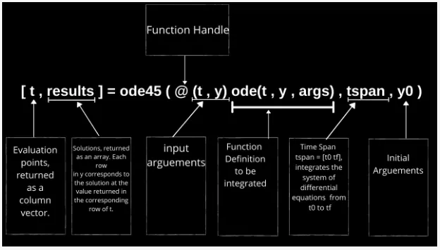
• Here we are using this ODE45 function to solve the differential equations
• below plot shows the angular displacement and angular velocity

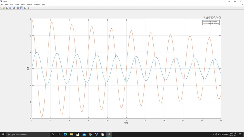
• Where in results first column repersents displacement and second column represents angular velocity

PROGRAME FOR THE SIMPLE PENDULUM ANIMATION

% pendulum animation

ct = 1
for i = 1:length(results(:,1))
x0 = 0;                      %coordinates for the fixed end of the pendulum
y0 = 0;

x1 = 1*sind(results(i,1));   %coordinates for the ball 
y1 = -1*cosd(results(i,1));


figure(2)

plot([-0.5 0.5],[0 0],'linewidth',3);
hold on
plot([x0 x1],[y0 y1],'linewidth',3,'color','r');
plot(x1,y1,'o','Markersize',50,'markerfacecolor','b');
hold off
axis([-0.2 0.2 -1.5 0]);
pause(0.01)
M(ct)=getframe(gcf);
grid on
ct = ct+1;

end
movie(M)
videofile = VideoWriter('Pendulum.avi','uncompressed avi');
open(videofile)
writeVideo(videofile, M)
close(videofile)

• Create a for loop where i = 1 to the length of 1st column of the result
• We are giving the x0 = 0 and y0=0 as the origin and also the fix end of the pendulum
• And then we have to give the positions for the ball

x1=1*sind(results(i,1))

y1=-1*cosd(results(i,1)) negitive is for the pendulum ball toward down

• In plot first line is to plot the line to which the pendulum is attached
• Give hold on after the first line because the first should not plot over and over
• And then plot a line from fixed to the ball [x1 y1]
• Create a marker of 'o' at the ball coordinates [x1 y1] and then hold off

• We will be getting the animation of simple pendulum to movie that we have to type M(ct)=getframe(gcf); after the pause and after 'for' loop end we have to type

• movie(M)
  videofile = VideoWriter('forward_kinematics.avi','uncompressed avi');
  open(videofile)
  writeVideo(videofile, M)
  close(videofile)

FINAL PROGRAM

close all 
clear all
clc

%inputs
l=1;                   %l = length of the pendulum in m,

m=1;                   %m = mass of the ball in kg,

b=0.05;                %b=damping coefficient.

g=9.81;                %g = gravity in m/s2,

%Time period
t_span = linspace(0,20,200);
  
%Displacement and initial velocity
theta_o = [0;3];

%ODE 
[t,results] = ode45(@(t,theta) ode_function(t,theta,b,m,g,l),t_span,theta_o);

figure(1)
plot(t,results(:,1))
hold on
plot(t,results(:,2))
ylabel('plot')
xlabel('time')
legend('displacement','angular velocity')


% pendulum animation

ct = 1
for i = 1:length(results(:,1))
x0 = 0;                      %coordinates for the fixed end of the pendulum
y0 = 0;

x1 = 1*sind(results(i,1));   %coordinates for the ball 
y1 = -1*cosd(results(i,1));


figure(2)

plot([-0.5 0.5],[0 0],'linewidth',3);
hold on
plot([x0 x1],[y0 y1],'linewidth',3,'color','r');
plot(x1,y1,'o','Markersize',50,'markerfacecolor','b');
hold off
axis([-0.2 0.2 -1.5 0]);
pause(0.01)
M(ct)=getframe(gcf);
grid on
ct = ct+1;

end
movie(M)
videofile = VideoWriter('Pendulum.avi','uncompressed avi');
open(videofile)
writeVideo(videofile, M)
close(videofile)

ERRORS FACED

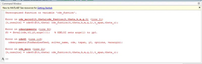
• While calling the function to the main program correct spelling should be given

• After plotting the first line we have to give the hold on to make the line should not over write for each value of the X1 Y1

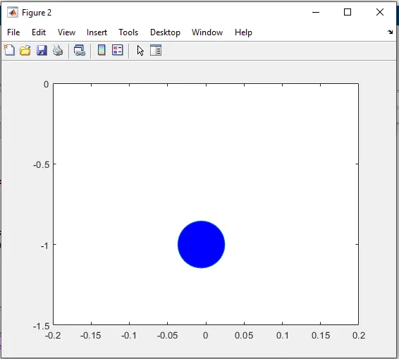
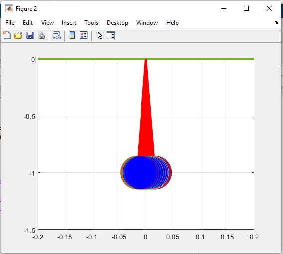
• After plotting we have to give the command hold off or else the plot will be plotted like this