Solving second order ODEs to simulate the motion of an ordinary Pendulum using MATLAB

Week 3 Report

• Aim: To write a code that solves the Ordinary Differential Equation that simulates the movement of an ordinary Pendulum.
  
  
  
  
  
• Introduction:
  
  A Pendulum is a body suspended from a fixed support so that it swings freely back and forth under the influence of gravity. When a pendulum is displaced sideways from its resting, equilibrium position, it is subject to a restoring force due to gravity that will accelerate it back toward the equilibrium position. When released, the restoring force acting on the pendulum's mass causes it to oscillate about the equilibrium position, swinging it back and forth. The mathematics of pendulums are in general quite complicated. Simplifying assumptions can be made, which in the case of a simple pendulum allow the equations of motion to be solved analytically for small-angle oscillations.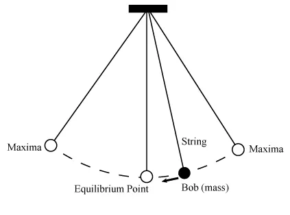
  
  
  
  
  Basic set up of a Pendulum.
  
  
  Now, we can get the
  
  The second order Differential Equation is in the following form: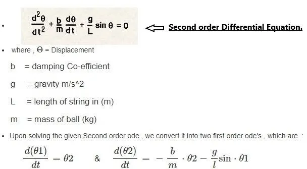
  
  
  
  
  
  here, b = Damping Coefficient
  
  g = Acceleration due to Gravity (m/s^2)
  
  L = Length of the Pendulum String (m)
  
  m = Mass of the ball. (kg)
  
  
  
  
  
  
  
  
  
  
  
• Code/Logic:
  
  1. We firstly need to clear and close all the previously entered codes and the preset values for any variables in it, hence we use the following commands:
  
  clear all
  close all
  clc
  
  
  
  2. In the next step, we must include the Inputs for the equation above:
  
  b = 0.05 (Damping coefficient)
  
  g = 9.81 (acceleration due to gravity)
  
  l = 1 (length of the pendulum)
  
  m= 1.0 (mass of the pendulum)
  
  
  
  3. Then, we define the timepoints at which the calculation will be done. This can be done by using the linspace command. In this command, we will specify the start time and the end time and the number of values that we want them to be divided into.
  
  
  4. In the next step, we must define the function in a new script, in which we split the Second Order Differential Equation into two simple first order differential Equation.
  We use two more variables and define them at the start of the function. We must use the two variables of theta1 and theta2 to define the following two Equation:
  
  `(d theta1) / (dt) = theta2`
  
  `(d theta2) / (dt) = - (b/m) * theta2 - (g /l) * sintheta1`
  
  We end the function by creating a solver vector.
  
  
  5. Next, we have to write the codes for the Plotting of the results and the animation. To plot the results, we must use the plot command. This command will basically plot the lines on a graph. So, we need to plot the lines between the time and the 1st column of the results.
  
  After the plotting is done, we then go onto stitch these plots together and create a movie from out of it. To do this, we simply have to assign a Variable (P in our case) and then assign all the frames to this variable. After all the variables were assigned, we then create a movie with this variable. We then have to create a Temporary Folder and then give the commands to open it and write and close the folder for this simulation. We can change the frame rate and other properties for the video as well.
  
  
  6. Then we must also write a code to define the position of the Pendulum ball. We start with the ball having no displacement and then we can give a marker of the shape of a circle to represent the ball. The code for the same is given below:.
  
  
  
  The main code is as follows:
  

  clear all
  close all 
  clc 
  
  %Inputs for the Equation:
  
  b = 0.05;         %b is the Damping coefficient
  g = 9.81;         %g is the acceleration due to gravity
  l = 1;            %l= length of the pendulum
  m= 1.0;           %m is the mass of the pendulum
  
  
  %Initial Condition
  theta = [0;3];    %0 is the initial displm and 3 is the Angular Velocity
  
  
  %Timepoints
  t_span = linspace (0,20,500);
  
  
  %Solving the ODE 
  [t,results] = ode45(@(t,theta) ode_func(t, theta, b,g,l,m), t_span, theta);
  
  
  %Plotting Graphs 
  plot(t,results(:,1))
  hold on 
  plot (t,results (:,2))
  ylabel('Plot')
  xlabel('Time')
  
  
  displ = results (:,1);
  
  %Code for the Pendulum
  ct =1 
  
  for i = 1:length(t)
   
      %Initial Position of Pendulum
      x0 =0 ;
      y0= 0;
      
      %Final Position of the Pendulum
      x1 = l*sin(displ(i));
      y1= -l*cos(displ(i));
      
      
      %Plotting 
      figure(2) 
      
      %Base line 
      plot([-1 1], [0 0], 'linewidth' ,2, 'color' ,'r')
      hold on
      
      %Pendulum String
     line ([x0 x1], [y0 y1], 'linewidth' ,2, 'color', 'b')
      
      %Pendulum Ball
      plot(x1, y1, 'marker', 'O', 'markersize' , 25)
      
      %Animation Plot
      axis ([-2 2 -2 2])
      pause = 0.2
      
      P(ct) = getframe(gcf)
      ct = ct+1
      hold off
      
  end 
       
  
  movie(P)
  videofile = VideoWriter ('Simple_Pendulum.avi' , 'uncompressed AVI')
  open(videofile)
  writeVideo (videofile,P)
  close(videofile)
  
  ​

  
  
  The function "ode_func" is also given below:
  

  function [dtheta_dt] = ode_func (t, theta, b,g,l,m)
  
  theta1 = theta(1)
  theta2 = theta (2)
  dtheta1_dt = theta2
  dtheta2_dt = -(b/m) * theta2 - (g/l) * sin(theta1)
  dtheta_dt = [dtheta1_dt; dtheta2_dt]
     
  end
  ​

  
  
  
  
  
  
  
  
  
  
  
• Results:
  
  We get the following Graph that shows the damping done on the pendulum: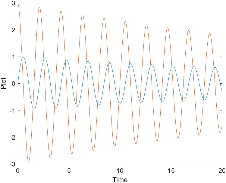
  
  
  
  Graph for Angluar Velocity and the Displacement of the Pendulum.
  
  
  The Blue line is the Displacement of the string and the orange line represents the Angular velocity of the Pendulum.
  
  
  
  
  The Animation of the Pendulum:
  
  
  
  
  
  
  
  
  
  
  
  
  
• Errors: The errors that I faced were majorly the typos and the parantheses while using specific commands. So, when MATLAB pointed out an error, I checked for the line number and then checked for any typos and corrected them right away.
  
  
  
  
  
  
  
  
• Conclusion: In conclusion, I would like to state that, this challenge helped me understand how to solve the Second Order Differential Equation for a simple Pendulum.