Solving second order ODEs (Pendulum)

Introduction: The motion of a pendulum is a very commonly studied phenomenon. It involves understanding the variation of angular velocity and angular displacement with respect to time.

The equation of motion for a pendulum is a second order differential equation.

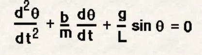
Here,

g = gravity in m/s2,

L = length of the pendulum in m,

m = mass of the ball in kg,

b=damping coefficient.

In this project, the pendulum motion is simulated and visualized using MATLAB.

Procedure

assumptions:

L=1 metre,

m=1 kg,

b=0.05.

g=9.81 m/s2.

Boundary conditions:

Time span 0-20 sec, for initial angular displacement=0, angular velocity=3 rad/sec at time t=0.

Code:

close all 
clear all
clc

b = 0.05;
g = 9.81;
l = 1;
m = 0.1;

%initial conditions
theta0 = [0;3]; %displacement, velocity

t_span = linspace(0,20,500); %time array, from 0 to 10 seconds

%solving the second order ode
[t,results] = ode45(@(t,theta) ode_func(t,theta,b,g,l,m),t_span,theta0);
                               %funct. to integrate    %initial conditions
figure(1)                                              %for ode_func(t,theta)
plot(t,results(:,1))
hold on
plot(t,results(:,2))
ylabel('plot')
xlabel('time')
ct = 0;
for i = 1:length(t)
    x0 = 0;
    y0 = 0;
    x1 = l*sin(results(i,1));
    y1 = -l*cos(results(i,1));
    
    figure(2)
    plot([x0,x1],[y0,y1]) %string of pendulum setup
    line([-1,1],[0,0],'linewidth',5,'color','r') %rod 
    
    hold on;
    
    plot(x1,y1,'o','markers',30,'markerfacecolor','y') %ball
   
    axis([-2 2 -2 2]);
    hold off;
    pause(0.01);
    ct = ct + 1;
    M(ct) = getframe(gcf)
    
end

movie(M)
videofile = VideoWriter('pendulum motion.avi','uncompressed AVI')
open(videofile)
writeVideo(videofile,M)
close(videofile)

It can be noted that an annonymous function ode45 is used.

This function basically requires the following inputs:

• A first order ODE equation.
• Time span
• Initial conditions

To provide ode45 with a first order ODE,

a seperate function is used.

In this function, the 2nd order differential equation of the pendulum is converted into 2 first order differential equations.

%this is the func that will be used by ode45 to solve the 2nd order ode
function [dtheta_dt] = ode_func(t,theta,b,g,l,m)
theta1 = theta(1); %angular dispacement
theta2 = theta(2); %angular velocity
dtheta1_dt = theta2;
dtheta2_dt = -(b/m)*theta2 - (g/l)*sin(theta1);
dtheta_dt = [dtheta1_dt;dtheta2_dt];
end

%ode45 solves the 2 1st order ode's stored in dtheta_dt

Here, what essentially happens is that the 2nd order equation is first split into two variables, theta1 and theta2.

dtheta1_dt and dtheta2_dt are the 2 first order ode's.

These values are solved by obtaining hand calculated equations to get dtheta1_dt and dtheta2_dt (Instead of actually differentiating). These values are stored in dtheta_dt which is fed into ode45 which solves the first order equations.

The output can be seen:

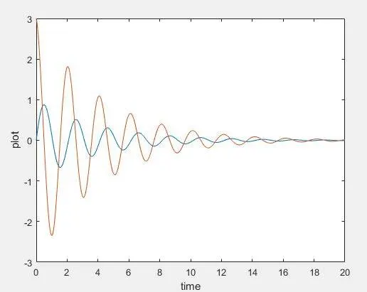
Pendulum motion:

https://drive.google.com/file/d/15YQ4ZtvtWLs5FiD5_A_ToxBUXvPpyDhW/view?usp=sharing