Solving second order ordinary differential equation

Introduction:

In Engineering, an Ordinary Differential Equation (ODE) is used to describe the transient behavior of a system. A simple example is a pendulum. The way the pendulum moves depends on Newton's second law. When this law is written down, we get a second-order ODE that describes the position of the suspended ball with respect to time.

Similarly, there are hundreds of ODE's that describe key phenomena, and if one has the ability to solve these equations it will be easy to simulate any of these systems.

Objectives:

1.) To write a program that solves the following ODE. This ODE represents the equation of motion of a simple pendulum with damping. The equation of motion of a simple pendulum is shown below.

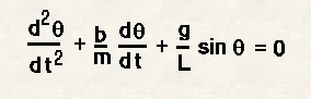
In the above equation:

g = gravity in m/`s^2`

L = length of the pendulum in m

m = mass of the ball in kg

b=damping coefficient

2.) Also, simulate the pendulum motion using

L=1 meter,

m=1 kg,

b=0.05.

g=9.81 m/s2.

Simulate the motion between 0-20 sec, for angular displacement=0,angular velocity=3 rad/sec at time t=0.

Software Used:

In order to achieve the above objective, we will be using MATLAB Software. MATLAB Software cannot directly solve the second-order equation given. So, we convert the second-order equation to two single order equations. After solving, the two single order equations come out to be as below.

`d theta1`/`dt`=`theta2`

`d theta2`/`dt`= -(b/m)*`theta2`-(g/l)*sin`theta1`

Code:

Program to create a function:

function[dtheta_dt]=functi(theta,t,b,g,l,m)
theta1=theta(1);
theta2=theta(2);
dtheta1_dt=theta2;
dtheta2_dt=-(b/m)*theta2-(g/l)*sin(theta1);
dtheta_dt=[dtheta1_dt;dtheta2_dt];
end

Main Program

clear all
close all
clc

% Inputs
b=0.05; % Damping coefficient
m=1; % Mass
g=9.81; % Gravity
l=1; % Length of the pendulum
theta=[0;3]; % Initial Conditions for displacement and velocity
t=linspace(0,20,500); % Time

% Solving using ODE function
[t, results]=ode45(@(t,theta) functi(theta,t,b,g,l,m),t,theta);

% Plotting time v/s displacement, time v/s velocity
figure(1)
plot(t,results(:,1))
hold on
plot(t,results(:,2))
hold off
xlabel('time')
ylabel('plot')
title('Time v/s Displacement and Time v/s Velocity plots')
grid on

% Plotting displacement v/s velocity
figure(2)
plot(results(:,1),results(:,2))
xlabel('displacement')
ylabel('velocity')
title('Displacement v/s Velocity plot')
grid on

% Plotting the movement of pendulum and creating movie
ct=1;
theta2=results(:,1);
for i=1:length(theta2)
theta_x=theta2(i);
x0=0;
y0=0;
x1=l*sin(theta_x);
y1=-l*cos(theta_x);
figure(3)
plot([-0.5 0.5],[0 0])
hold on
plot([x0 x1],[y0 y1])
hold on
plot(x1,y1,'o','markers',15,'markerfacecolor','g');
hold off
grid on
title('Pendulum Animation')
axis([-1.5 1.5 -1.5 0.5])
M(ct)=getframe(gcf);
ct=ct+1;
end

movie(M)
videofile=VideoWriter('pendulum_ode.avi','uncompressed avi');
open(videofile)
writeVideo(videofile,M)
close(videofile)

Output:

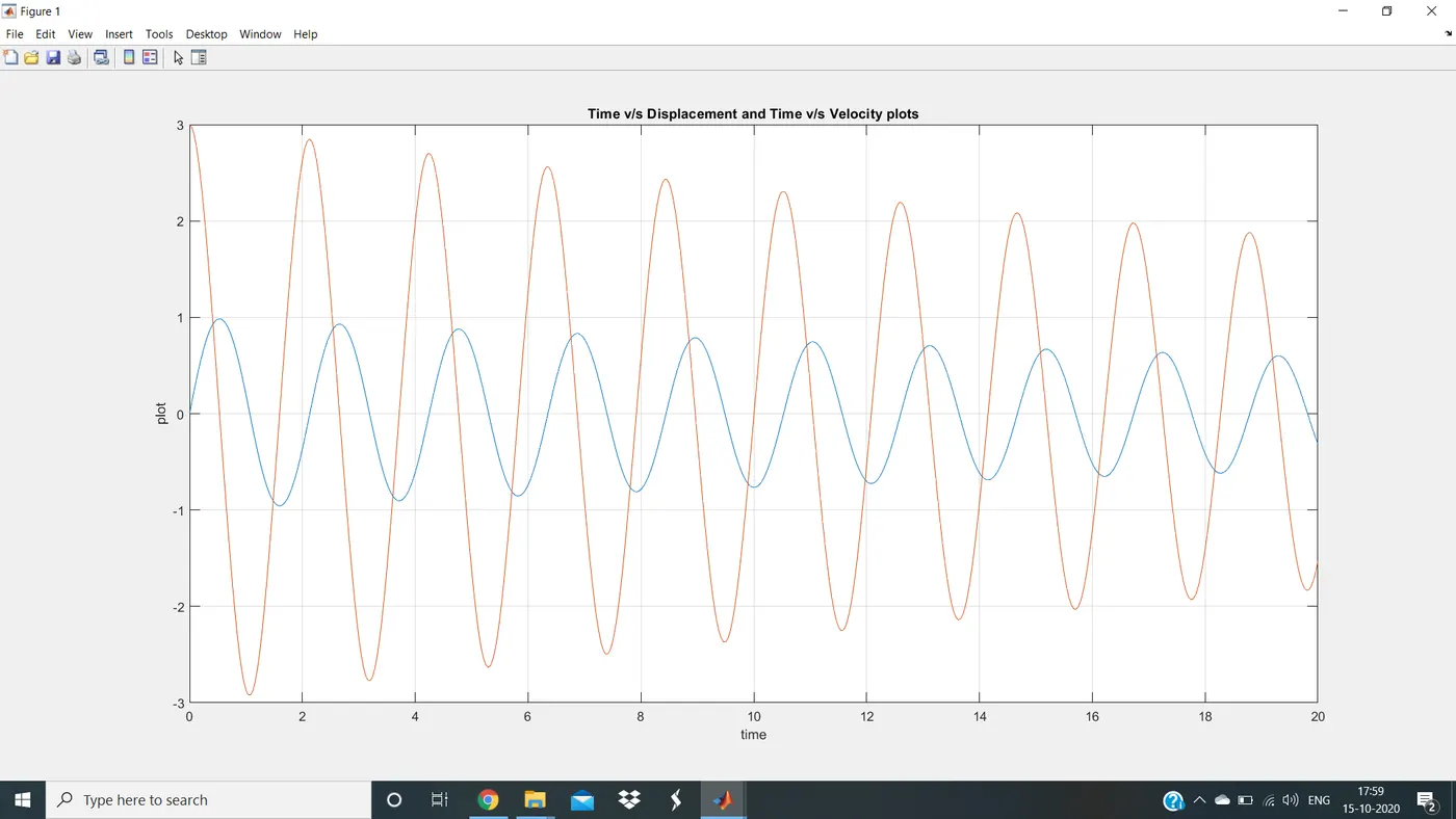
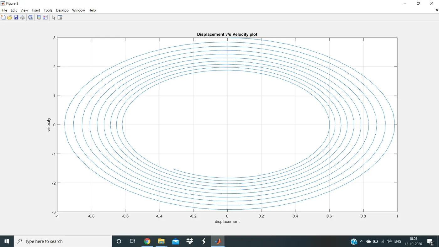
Video simulating the pendulum motion: https://drive.google.com/file/d/1mqsglv2o07lM-nKoXjo79SYFY2EcmFZp/view?usp=sharing