Curve fitting

Objectives:

• To write code to fit a linear and cubic polynomial for the cp data.
• Plot the linear and cubic fit curves along with the raw data points.
• To write a code to show splitwise method.
• To explain the parameters used to measure the fitness characteristics for both the curves.

Also, answer the following questions:

1. How to make a curve fit perfectly?
2. How to get the best fit? Note: Best fit and perfect fit are two completely different phenomena.
3. What could be done to improve the cubic fit?

Software Used: MATLAB

Theory:

Curve fits are really useful as they help us describe how the data changes mathematically. Once we have a curve fit, we can do additional mathematical operations which might not be possible in the initial data set. For example, if you do a curve fit for population variation with time data, you will get a mathematical function in which you can put a future time and predict what the population is going to be.

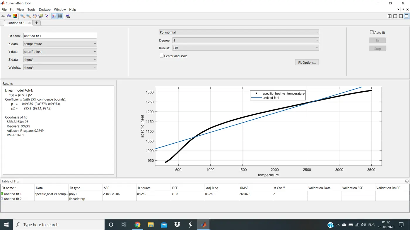
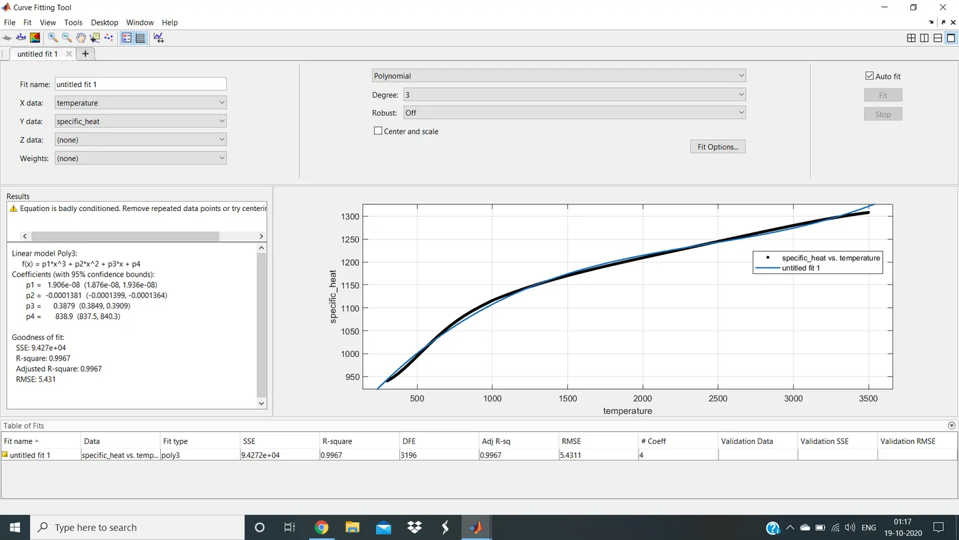
With a curve fit, usually, we can get some rough trends. And since the curve fit is basically a mathematical function, we can also do additional operations like taking derivatives and so on. The parameters used to measure the goodness of fit between the two curves are, the sum of squares due to error (SSE), R-square, adjusted R-square, root mean square error (RMSE).

The Sum of squared error measures the total deviation of the response values from the fit to the response values.

R-square is the square of the correlation between the response values and the predicted response values.

Adjusted R-square uses the R-square statistic defined above, and adjusts it based on the residual degrees of freedom. The residual degrees of freedom is defined as the number of response values n minus the number of fitted coefficients m estimated from the response values.

Root mean square error is an estimate of the standard deviation of the random component in the data.

In order to make a perfect fit, we must consider error estimates as well. A perfect fit means, the curve should fit the original curve without showing any errors (such as centering and scaling errors) in that particular degree of the polynomial. A perfect fit can always be the best fit but the best fit can not be a perfect fit. The best fit can be achieved by using interpolant in curve fitting toolbox or by using the splitwise method discussed below.

Dataset: Here, we will take up the data containing specific heat for oxygen as a function of time. In this dataset, the first column is temperature and the second column is specific heat. To load the dataset, we need to make sure that the dataset is present in the same directory as the program. To check the location of the program, type 'pwd' in the command window. Click here to download the dataset.

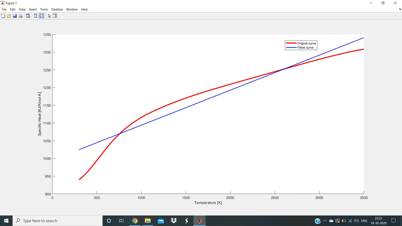
Code to fit linear polynomial for the data:

% Program to fit linear polynomial for the data

clear all
close all
clc

% Loading the data
cp_data=load('data');

% Defining the data
temperature=cp_data(:,1);
specific_heat=cp_data(:,2);

% Calculating coefficients and predicted specific heat
coeff=polyfit(temperature,specific_heat,1);
predicted_specific_heat=polyval(coeff,temperature);

% Plotting
hold on
plot(temperature,specific_heat,'linewidth',3,'color','r');
plot(temperature,predicted_specific_heat,'linewidth',2,'color','b');
xlabel('Temperature [K]');
ylabel('Specific Heat [KJ/Kmol-K]');
legend('Orignal curve','Fitted curve');

Output of code to fit linear polynomial for the data:

Goodness of fit for above plot:

Code to fit cubic polynomial for the data:

% Program to fit cubic polynomial for the data

clear all
close all
clc

% Loading the data
cp_data=load('data');

% Defining the data
temperature=cp_data(:,1);
specific_heat=cp_data(:,2);

% Calculating coefficients and predicted specific heat
coeff=polyfit(temperature,specific_heat,3);
predicted_specific_heat=polyval(coeff,temperature);

% Plotting
hold on
plot(temperature,specific_heat,'linewidth',3,'color','r');
plot(temperature,predicted_specific_heat,'linewidth',2,'color','b');
xlabel('Temperature [K]');
ylabel('Specific Heat [KJ/Kmol-K]');
legend('Orignal curve','Fitted curve');

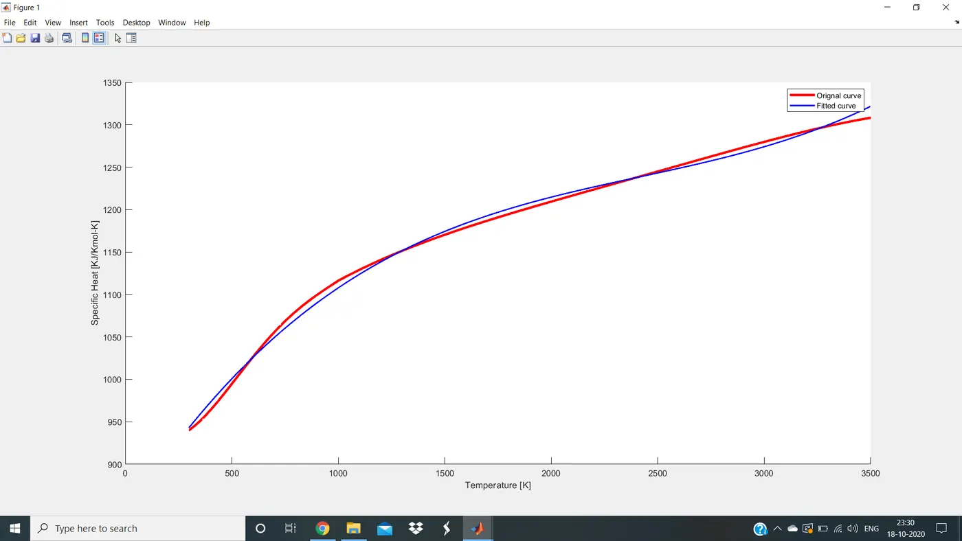
Output of code to fit cubic polynomial for the data:

Goodness of fit for the above plot:

From the above figure, it can be inferred that the fitted curve seems to be closely resembling the original curve. We can improve the fitted curve further to bring it even closer to the original curve. This can be done using splitwise method where we split the curves and try to make the fitted curve resemble the original curve as closely as we can.

Code for Splitwise Method:

% Program to perform splitwise fit for the data

clear all
close all
clc

% Loading the data
cp_data=load('data');

% Defining the data
temperature1=cp_data(1:1500,1);
temperature2=cp_data(1501:3200,1);
specific_heat1=cp_data(1:1500,2);
specific_heat2=cp_data(1501:3200,2);

% Calculating coefficirnts and predicted specific heat
coeff13=polyfit(temperature1,specific_heat1,3);
coeff23=polyfit(temperature2,specific_heat2,3);
predicted_specific_heat13=polyval(coeff13,temperature1);
predicted_specific_heat23=polyval(coeff23,temperature2);

% Plotting
hold on
plot(temperature1,specific_heat1,temperature2,specific_heat2,'linewidth',3,'color','r');
plot(temperature1,predicted_specific_heat13,temperature2,predicted_specific_heat23,'linewidth',1,'color','g');
xlabel('Temperature [K]');
ylabel('Specific Heat [KJ/Kmol-K]');
legend('Orignal curve Part 1','Orignal curve Part 2','Fitted Curve Part 1','Fitted Curve Part 2');

Output for splitwise method:

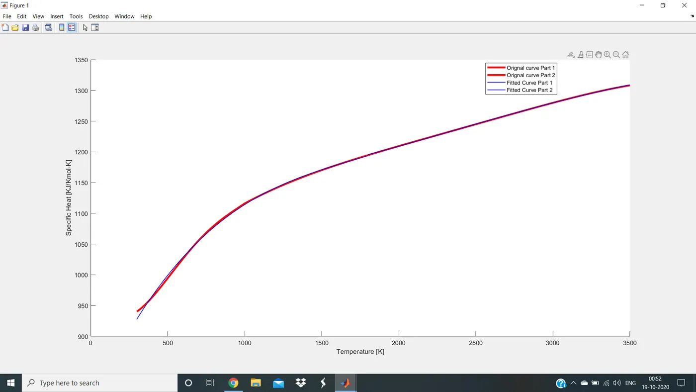
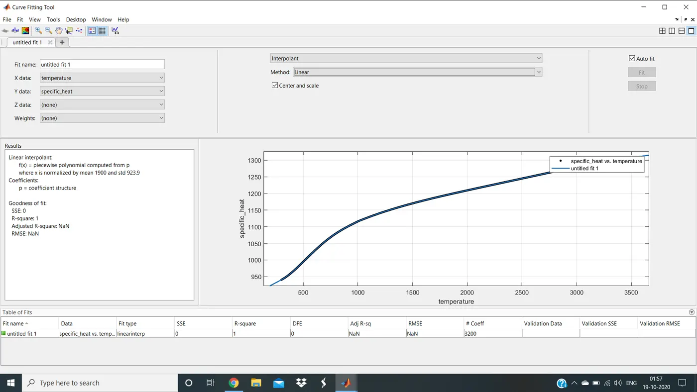
Using multiple splits can sometimes be too tedious. A simpler and more efficient method would be using interpolant in the curve fitting tool for the same data as above.

Output for using the interpolant in curve fitting tool:

References:

https://in.mathworks.com/help/curvefit/evaluating-goodness-of-fit.html

https://in.mathworks.com/matlabcentral/answers/349776-how-to-find-the-best-curve-fit-for-a-set-of-data

https://skill-lync.com/projects/Week-4-Curve-fitting-31550#:~:text=In%20order%20to%20make%20perfect,not%20be%20a%20perfect%20fit.