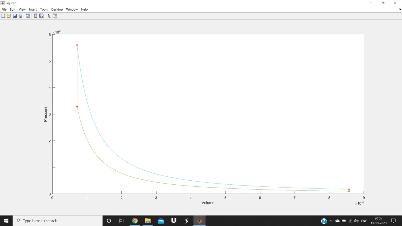
Air standard cycle

Aim: To write code that can solve an otto cycle and make plots for it.

Requirement: Code should create a PV diagram.

Software Used: MATLAB

Theory:

Air standard cycles are pretty important. They help us understand the theoretical limits of a particular cycle which can be used to get an idea about the performance of real-world systems like IC engines or turbines. Here we will be writing a program that actually simulates the otto cycle. Once learned the complete program, it will become easy to solve any other air standard cycle. The typical P-V diagram for the otto cycle looks as shown below:

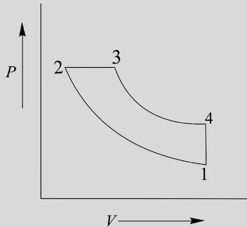
1-2 Isentropic compression

2-3 Constant volume heat addition

3-4 Isentropic expansion

4-1 Constant volume heat rejection

Let us talk about the inputs that are typically provided and how to solve the problem.

• Typically, volume at state 1 (v1), the temperature at state 1 (t1) are provided directly or indirectly. In this case, instead of starting with v1 directly, we are going to start with engine geometric parameters. Once we have these parameters, we will be able to solve the kinematics equation and compute the volume traced. Volume traced can help us to calculate swept volume and clearance volume with which we can calculate v1.
• With v1, t1, we can find out pressure at state 1 (p1).
• The other input that is typically provided is the compression ratio (cr).
• With cr, v2 can be calculated which in turn can be used to calculate p2 which in turn can be used to calculate t2.
• Usually, in these type of problems, the temperature or pressure after combustion is also provided which mean either t3 is provided or p3 is provided. In this case, we are going to assume that t3 is provided.
• t3 is known. v3 is also known (because v2 and v3 are going to be the same because of constant volume heat addition).
• Once t3 and v3 are known, p3 can also be calculated. A similar concept can be applied and we can calculate the values for state 4. Once we have all this information, it is easy to plot 4 points in our P-V diagram.
• Now, we cannot simply connect these points with straight lines because that would be incorrect.
• In order to determine the paths correctly, we need to know the thermodynamic relationship during compression using piston kinematics.

Code:

% Engine Kinematics Function Program.

% This is a MATLAB program that is saved in the same folder as the below program. 
% For the execution of the below program, save this program before trying to execute
% the below program.

function[v]=engine_kinematics(bore,stroke,con_rod,cr,start_crank,end_crank)

% There is a specific equation to calculate the value of v. It is
% v=(1+0.5(cr-1)*{(R+1-cosd(theta)-[(R^2-sind(theta)^2]^0.5}*v_c
% Below we have provided all the inputs to facilitate the calculation of v.
% We have calculated the value of v for different values of theta. These
% values are stored in an array. It would be very confusing for us to
% directly put up the above formula of v. So, we split the formula into
% three terms and combined all the terms as shown below.

a=stroke/2;
R=con_rod/a;
v_s=(pi/4)*bore^2*stroke;
v_c=v_s/(cr-1);
theta=linspace(start_crank,end_crank,100);
term1=0.5*(cr-1);
term2=R+1-cosd(theta);
term3=(R^2-sind(theta).^2).^0.5;
v=(1+term1*(term2-term3)).*v_c;

end

% Otto Cycle Using MATLAB

clear all
close all
clc

% Input variables
gamma=1.4;
p1=101325; % Pressure=1atm=101325 pascal (all pressures are in pascal)
t1=500; % Temperature=500K (all temperatures are in kelvin)
t3=2300;

% Engine geometric parameters
bore=0.1;
stroke=0.1;
con_rod=0.15;
cr=12;

% Calculation of swept volume and clearance volume
v_swept=(pi/4)*bore^2*stroke;
v_clearance=v_swept/(cr-1);

v1=v_swept+v_clearance;
v2=v_clearance;

% p1*v1^gamma=p2*v2^gamma. Therefore
p2=p1*cr^gamma; %cr=v1/v2

% p1*v1/t1=p2*v2/t2. Therefore
t2=p2*v2*t1/(p1*v1);

% Since the process from 2-3 is constant volume heat addition
v3=v2;

% p3*v3/t3=p2*v2/t2. Therefore
p3=p2*t3/t2;

% Since the process from 4-1 is a constant volume heat rejection
v4=v1;

% p3*v3^gamma=p4*v4^gamma. Therefore
p4=p3*(v3/v4)^gamma;

% p3*v3/t3=p4*v4/t4. Therefore
t4=p4*v4*t3/(p3*v3);

% Engine_kinematics is the function we have created
constant_c1=p1*v1^gamma;
% The process is compression. Therefore theta varies from 180 to 0
v_compression=engine_kinematics(bore,stroke,con_rod,cr,180,0);
p_compression=constant_c1./v_compression.^gamma;
constant_c2=p3*v3^gamma;
% The process is expansion. Therefore theta varies from 0 to 180
v_expansion=engine_kinematics(bore,stroke,con_rod,cr,0,180);
p_expansion=constant_c2./v_expansion.^gamma;

% Plotting the Otto cycle
hold on
plot(v1,p1,'*','color','r');
plot(v2,p2,'*','color','r');
plot(v3,p3,'*','color','r');
plot(v4,p4,'*','color','r');
plot(v_compression,p_compression);
plot(v_expansion,p_expansion);
plot([v2 v3],[p2 p3]);
plot([v1 v4],[p1 p4]);
xlabel('Volume')
ylabel('Pressure')

Output: