Simulation of forward kinematics of a 2R robotic arm

Aim: To write a program to simulate the forward kinematics of a 2R Robotic Arm.

Software Used: MATLAB.

Theory:

When one gets started with robotics, the first thing that is taught is the kinematics of linkages. It has a lot of applications. Figuring out how the robot is going to move helps us identify its workspace. Workspace refers to all possible locations that the robot can reach. Knowing the workspace is really important when people are designing robots for really complex applications such as welding a complex frame.

Let us look at a 2R robotic arm shown below:

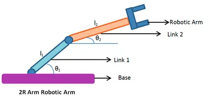
The 2R robotic arm consists of a base, 2 links and 2 rotational joints. Here, link 1 makes an angle of θ1 with respect to the x-axis and link 2 makes an angle θ2 with respect to the x-axis. Also, the length of link 1 is l1 and the length of link 2 is l2.

Problem: So, with respect to forward kinematics, the problem reduces to the following:

If θ1 and θ2 are given, what is the final position of the manipulator?

Solution: Below is a MATLAB program to find a solution to the above problem. The code contains comments at every step which shall guide you to understand the logic.

% Forward kinematics of a 2R robotic arm
clear all
close all
clc
% This robotic arm has two links l1 and l2. The sizes of links are
% considered as follows
l1=1;
l2=0.5;
% theta1 represents the angles link 1 can make with the x-axis
% theta2 represents the angles link 2 can make with the x-axis
theta1=linspace(0,90,4);
theta2=linspace(0,90,4);
% Here for every one position of link 1, link 2 can have 4 different
% positions. Eg: For theta1=0, we can have theta2=0/30/60/90. In order to
% potray this,we are using two for loops one inside another as shown.
ct=1;
for i=1:length(theta1)
THETA1=theta1(i);
for j=1:length(theta2)
THETA2=theta2(j);
% (x0,y0) lie at origin. (x0,y0) represent the starting position of
% link 1
x0=0;
y0=0;
% The formulae for (x1,y1) are as follows. (x1,y1) represents the
% end position of link 1 and starting position of link 2
x1=l1*cosd(THETA1);
y1=l1*sind(THETA1);
% The formulae for (x2,y2) are as follows. (x2,y2) represent the
% end position of the link 2
x2=x1+l2*cosd(THETA2);
y2=y1+l2*sind(THETA2);
% We use plot command along with pause to get the animation as
% desired. The width of the lines in the plot is set to 3.
plot([x0 x1],[y0 y1],[x1 x2],[y1 y2],'linewidth',3);
pause(0.7)
% Our axis is changing in output. So to fix our axis, we used below
axis([-0.2 2 -0.2 2])
% We get our frames and the frames are stored in an array called M
M(ct)=getframe(gcf);
% After the frame is stored in array, the counter is increased and
% next frame is fetched and stored and so on.
ct=ct+1;
end
end
% All the frames stored in the array M are converted into a movie using
movie(M)
% We create a videofile and name it using command below
videofile=VideoWriter('Challenge_Robot.avi','uncompressed avi');
% Then we open the videofile
open(videofile)
% We insert our video in the videofile
writeVideo(videofile,M)
% Then we close the video file using the command below
close(videofile)

Output: The output of the program gives information about the workspace which is really important when people are designing robots for really complex applications such as welding a complex frame. The link to the output animated video is posted below.

https://drive.google.com/file/d/1umiUyHue5ALNeOy-d8QEyBbOwOoM_Y7H/view?usp=sharing