Parsing NASA thermodynamic data

Introduction:

NASA came up with polynomials that can be used to evaluate thermodynamic properties such as specific heat, enthalpy and entropy. They have also documented the coefficients that are required to evaluate these polynomials for 1000+ species. The documented coefficients can be found here in NASA thermodynamic data file and the polynomials are as follows:

Objectives:

1. Write a function that extracts the 14 coefficients and calculates the enthalpy, entropy and specific heats for all the species in the data file. We will be working with this file NASA thermodynamic data. In this file, R is the universal gas constant, T is the temperature. The first 7 coefficients of each species are high-temperature coefficients and the second 7 coefficients of each species are low-temperature coefficients.
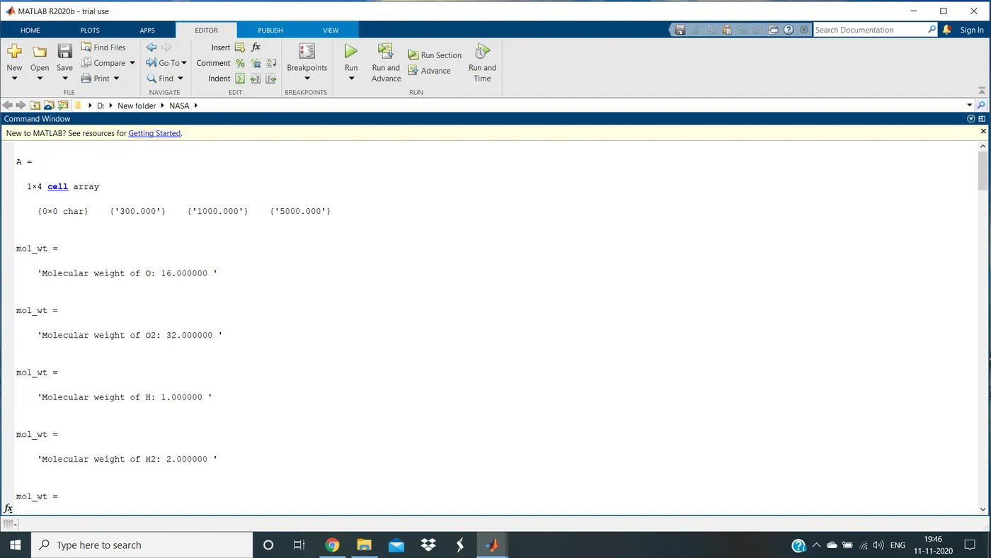
2. Calculate the molecular weight of each species and display it in the command window.
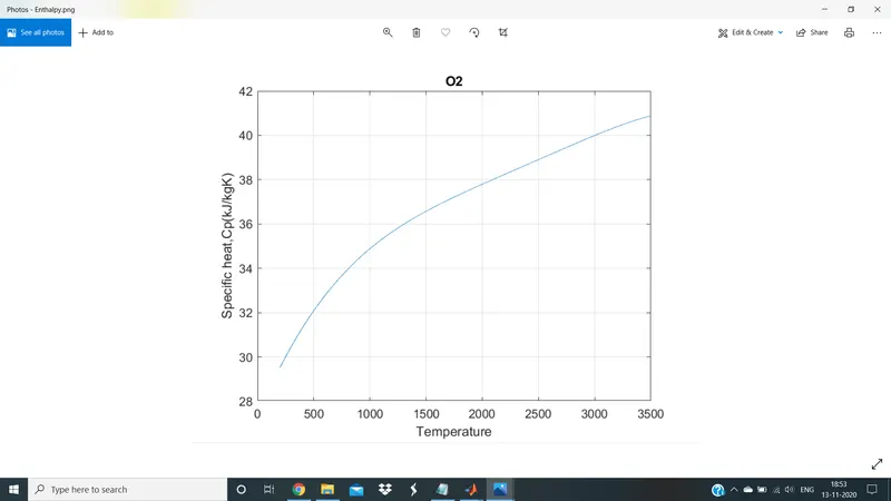
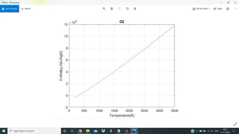
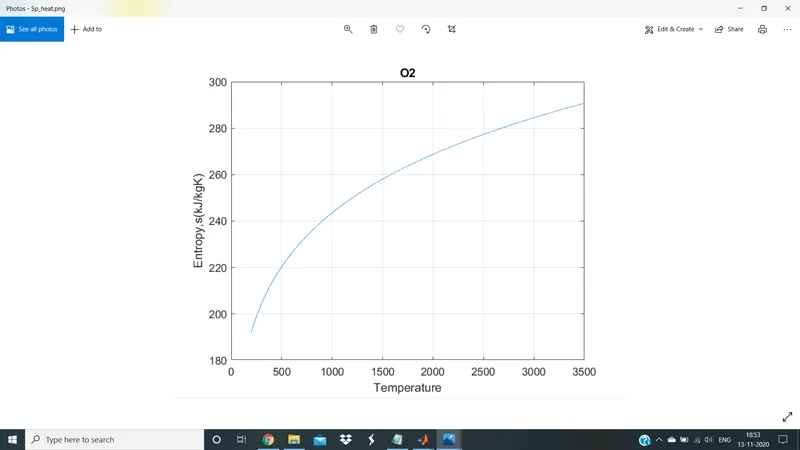
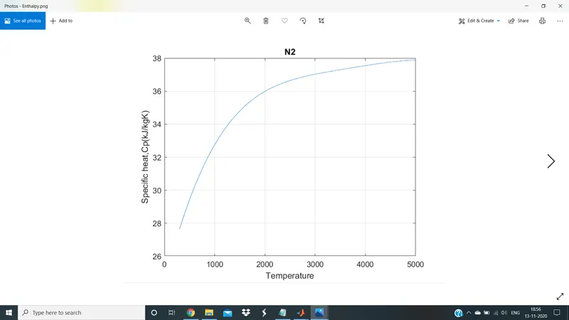
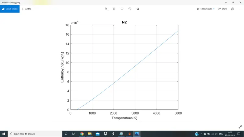
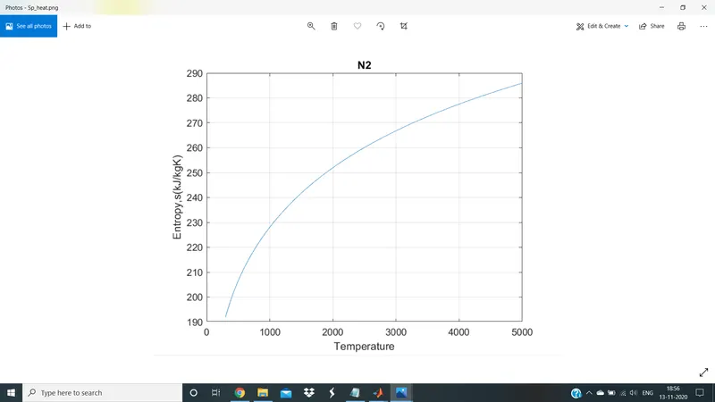
3. Plot the specific heat, enthalpy and entropy for the local temperature range (low temperature: high temperature) specific for each species.
4. Save the plots as images with appropriate names and dump them in separate folders for each species with a suitable name. All of these should be generated automatically.

Software Used: MATLAB

Code:

clear all
close all
clc

fid=fopen('thermo.dat','r');
%checking for the sign of file identifier
if fid<0
    fprint('there is an error, fid can''t be negative. end./n')
end

Header=fgetl(fid);
% getting the global low, mid, and high temperatures as a string
tline=fgetl(fid); 
fgetl(fid);   % ignorning the comment lines
fgetl(fid);
fgetl(fid);

A=strsplit(tline,' ')  %getting tht global low, med and high as numbers
global_low_temp=str2num(A{2});
global_mid_temp=str2num(A{3});
global_high_temp=str2num(A{4});


for i=1:53
%getting the first line of a species as a string

line_1=fgetl(fid);    
x=strsplit(line_1,' ');
species_name=x{1};%getting species names
z=length(x);
local_low_temp=str2double(x{z-3}); %storing the temp values as numbers
local_mid_temp=str2double(x{z-1});
local_high_temp=str2double(x{z-2});

t1=local_low_temp;
t2=local_mid_temp;
t3=local_high_temp;

%getting a1-a5 coeff

line_2=fgetl(fid); %getting the second line of the species
find_E=findstr(line_2,'E');   % creating a vector of 'E' index     

a1=line_2(1:find_E(1)+3); %using position of 'E' to get a1 as string
a1=str2num(a1); %converting a1 to num and storing it back in a1

a2=line_2(find_E(1)+4:find_E(2)+3); 
a2=str2num(a2);

a3=line_2(find_E(2)+4:find_E(3)+3); 
a3=str2num(a3);

a4=line_2(find_E(3)+4:find_E(4)+3); 
a4=str2num(a4);

a5=line_2(find_E(4)+4:find_E(5)+3); 
a5=str2num(a5);

%getting a6-a10

line_3=fgetl(fid);   % same as a1-a5 except now it is line 3 and coeff a6-a10
find_E=findstr(line_3,'E');     

a6=line_3(1:find_E(1)+3); 
a6=str2num(a6); 

a7=line_3(find_E(1)+4:find_E(2)+3); 
a7=str2num(a7);

a8=line_3(find_E(2)+4:find_E(3)+3); 
a8=str2num(a8);

a9=line_3(find_E(3)+4:find_E(4)+3); 
a9=str2num(a9);

a10=line_3(find_E(4)+4:find_E(5)+3); 
a10=str2num(a10);

%getting a11-a14 coeff

line_4=fgetl(fid) ;  
find_E=findstr(line_4,'E');

a11=line_4(1:find_E(1)+3); 
a11=str2num(a11); 

a12=line_4(find_E(1)+4:find_E(2)+3); 
a12=str2num(a12);

a13=line_4(find_E(2)+4:find_E(3)+3); 
a13=str2num(a13);

a14=line_4(find_E(3)+4:find_E(4)+3); 
a14=str2num(a14);

% creaing a new folder with species name to store its plots
mkdir(species_name)
cd(species_name)

T = linspace(t1,t3,1000);
R=8.314;
for j=1:length(T)
    % a1-a7 ---> high temp coeff
    if T(j)>t2  %comparison with mid temp
        
    Cp=(a1+a2.*T+a3.*T.^2+a4.*T.^3+a5.*T.^4)*R;     % calc of Cp, h and s
    h=(a1+(a2.*T)/2+(a3.*T.^2)/3+(a4.*T.^3)/4+(a5.*T.^4)/5+(a6./T))*R.*T;
    s=(a1.*log(T)+a2.*T+(a3.*T.^2)/2+(a4.*T.^3)/3+(a5.*T.^4)/4+a7)*R;
    
    else  % low temp coeff
        Cp=(a8+a9.*T+a10.*T.^2+a11.*T.^3+a12.*T.^4)*R;     % calc of Cp, h and s
    h=(a8+(a9.*T)/2+(a10.*T.^2)/3+(a11.*T.^3)/4+(a12.*T.^4)/5+(a13./T))*R.*T;
    s=(a8.*log(T)+a9.*T+(a10.*T.^2)/2+(a11.*T.^3)/3+(a12.*T.^4)/4+a14)*R;
    end
       
end


 %plotting the 3 graphs
    figure(1)   %spc heat vs temp
    plot(T,Cp);
    grid on
     title(species_name);
    ylabel('Specific heat,Cp(kJ/kgK)');
    xlabel('Temperature');
    
    figure(2)
    plot(T,h); 
    grid on 
     title(species_name);
    ylabel('Enthalpy,h(kJ/kgK)');  % enthalpy vs temp
    xlabel('Temperature(K)');
    
    figure(3)
    plot(T,s); %entropy vs temp
    grid on
     title(species_name);
    ylabel('Entropy,s(kJ/kgK)');
    xlabel('Temperature');
    
    %changing directory and saving the file
    saveas(1,'Enthalpy.png')
    saveas(2,'Entropy.png')
    saveas(3,'Sp_heat.png')
    cd  ..   

    %mol wt calc
    atoms=['H','C','O','N','R']; % elements name for comparision
atomic_weight=[1 12 16 14 40]; % weight assigned to each element
MW=0;
for i=1:length(species_name)
    for j=1:length(atoms)
        if strcmp(species_name(i),atoms(j))
            MW=MW+atomic_weight(j);
            position=j; % storing position for reference outside loop
        end
    end
    n=str2num(species_name(i));
    if n>1
        MW=MW+atomic_weight(position)*(n-1); % adding extra atom's weight
    end
end
    mol_wt=sprintf('Molecular weight of %s: %f ',species_name,MW)
    % to display all the molecular weights in cammand window
end
  

Basic logical explanation of the program:

• First, we open the thermo.dat file to read. Then we skip through the first line which just reads THERMO.
• Then we go to the next line where global minimum, maximum and mid values are present. In this line ' ' (space) is the differentiator between each of the values.
• Hence, we use ' ' (space) to split the string using strsplit command and the split string is assigned with a variable global_temp. Low, mid and high of global_temp is calculated.
• Since all the data in the THERMO.dat file is stored in the form of a string, each value of global_temp is converted to a number using the str2num command and is assigned variables as shown in the code above.
• Then we skip the next 3 lines using fgetl(f1) as these lines just appear to be comments.
• Now we have extracted the header information. Next, we will be extracting the information of all the species. In this process, the first line of the species is extracted and is named before the name of the species using the strtok command. Command strtok returns the selected part of the string. Similar procedure as global_temp is done for achieving local_temp.
• Then we have defined the range of local_temp with 1000 values which lie between local_low_temp and local_high_temp. We have achieved this using linspace command.
• Then we define the universal gas constant i.e. R=8.314
• We will just be writing the code to extract the information from 1 species. To extract the information from all the species, we run the same code in 'for loop' for 53 times in order to extract the information from 53 species.
• In global_temp, we have used ' ' (space) to split the string. Here we will be using E to identify where the coefficient is ending and where a new coefficient is starting. Usually in a line, a particular coefficient ends 3 digits after E and a new coefficient starts 4 digits after E. This logic is used to split the coefficients in the species.
• First, 7 coefficients in the species are higher temperature coefficients and are assigned variables a1,a2,...,a7.
• The next 7 coefficients in the species are lower temperature coefficients and are assigned variables a8,a9,...,a14.
• Finally, specific heat, enthalpy, entropy, molecular weight calculations and plotting are done in accordance with their respective functions.

Logic explanation for calculating specific heat, enthalpy and entropy :

• The formulae to calculate specific heat, enthalpy and entropy respectively are the same as the polynomials shown above.
• One thing to note is that, if T>local_mid_temp, then higher temperature coefficients a1,a2,...,a7 are used. Else, lower temperature coefficients a7,a8,...,a14 are used.

Logic explanation for calculating molecular weight:

• Let us understand the logic of the above program using an example. Let us consider the example of O2 in this case.
• Atoms with their respective atomic weights are provided.
• Initially, the molecular weight is set to zero.
• Then we have a 'for loop i' which runs from 1 to the length of the species name (for O2, length of the name is 2). So, 'i' runs from 1 to 2. (The result for i=1 is O and for i=2, the result is 2)
• In the 'for loop i' we have another 'for loop j'. 'For loop j' runs from 1 to the length of atoms. In this case, the length of the atoms is 5 which consists of H, C, O, N and R.
• Then we have the strcmp command which compares species_name(i) and atoms(j).
• For i=1 and j=1, species_name(i)=O, atoms(j)=H. These are not the same and the loop continues with i=1 and j=2. species_name(i)=O, atoms(j)=C. These are again not the same and the loop continues.
• With i=1 and j=3. Here we get, species_name(i)=O, atoms(j)=O. Both are the same and hence MW=MW+atomic_weight(j) which is MW=MW+atomic_weight(3) which inturn is equal to 0+16=16.
• Then the value j=3 is stored in a variable called position. This continues until i=1 and j=5.
• Next, the value of i is changed. The value of i=2 is 2. Here, the value of i is greater than 1 but still in the form of a string. So, we convert this value in form of a string to a number using the str2num command and store it as n. Here, the value of n is 2. Then the value of molecular weight changes to MW=MW+atomic_weight(position)*(n-1). This gives us MW=16+atomic_weight(3)*(2-1) =16+16*1 =32.
• 32 is the output (molecular weight) for O2 and it is printed out.

Logic explanation to create plots:

• mkdir(species_name) command is used to create a new folder with the name same as the species name.
• And the plots that are created using the plot command are saved into the newly created folder using the command cd(species_name).
• Each figure is assigned a specific name and format using the saveas command.
• Finally, we use 'cd ..' to come out of the folder we were in and create another folder for later iterations of the loop. If we do not do this, the folder from the next iteration will be created in the first folder and so on.

Output:

Molecular Weight of each species displayed in command window:

Plots for (specific heat,enthalpy and entropy) vs (local temperature range) for each species are shown below.

Oxygen:

Nitrogen:

Carbon di oxide:

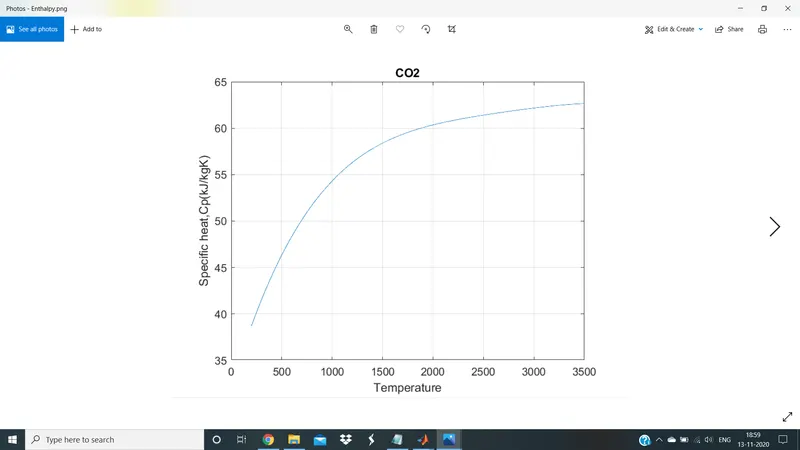
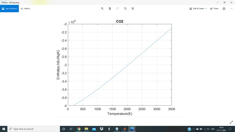
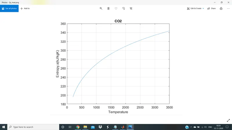
In a similar fashion, we have programmed MATLAB to generate 3 plots for each of the 53 species in the dataset. The plots of each species are organized in folders as shown below.